Statistics


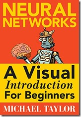
bookcover

Gradient Boosting Algorithm is one of the powerful algos out there for solving classification and regression problems.This book gives a gentle introduction to the various aspects of the algo with out overwhelming the reader with the detailed math of the algo. The fact that there are a many visuals in the book makes the learning very sticky. Well worth a read for any one who wants to understand the intuition behind the algo.

Here is a link to a detailed summary :

Machine Learning With Boosting – Summary


COVER

The author says that there are five things about Neural Networks that any ML enthusiast should know:

  1. Neural Networks are specific : They are always built to solve a specific problem
  2. Neural Networks have three basic parts, i.e. Input Layer, Hidden Layer and Output Layer
  3. Neural Networks are built in two ways
    • Feed Forward : In this type of network, signals travel only one way, from input to output. These types of networks are straightforward and used extensively in pattern recognition
    • Recurrent Neural Networks: With RNN, the signals can travel in both directions and there can be loops. Even though these are powerful, these have been less influential than feed forward networks
  4. Neural Networks are either Fixed or Adaptive : The weight values in a neural network can be fixed or adaptive
  5. Neural Networks use three types of datasets. Training dataset is used to adjust the weight of the neural network. Validation dataset is used to minimize overfitting problem. Testing dataset is used to gauge how accurately the network has been trained. Typically the split ratio among the three datasets is 6:2:2

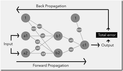
There are five stages in a Neural Network and the author creates a good set of visuals to illustrate each of the five stages:

  1. Forward Propagation
  2. Calculate Total Error
  3. Calculate the Gradients
  4. Gradient Checking
  5. Updating Weights

image

Be it a convolution neural network(CNN) or a recurrent neural network(RNN), all these networks have a structure-or-shell that is made up of similar parts. These parts are called hyperparameters and include elements such as the number of layers, nodes and the learning rate.Hyperparameters are knobs that can tweaked to help a network successfully train. The network does not tweak these hyperparameters.

There are two types of Hyperparameters in any Neural Network, i.e. required hyperparameters and optional hyperparameters. The following are the required Hyperparameters

  • Total number of input nodes. An input node contains the input of the network and this input is always numerical. If the input is not numerical, it is always converted. An input node is located within the input layer, which is the first layer of a neural network. Each input node represents a single dimension and is often called a feature.
  • Total number of hidden layers. A hidden layer is a layer of nodes between the input and output layers. There can be either a single hidden layer or multiple hidden layers in a network. Multiple hidden layers means it is is a deep learning network.
  • Total number of hidden nodes in each hidden layer. A hidden node is a node within the hidden layer.
  • Total number of output nodes. There can be a single or multiple output nodes in a network
  • Weight values. A weight is a variable that sits on an edge between nodes. The output of every node is multiplied by a weight, and summed with other weighted nodes in that layer to become the net input of a node in the following layer
  • Bias values. A bias node is an extra node added to each hidden and output layer, and it connects to every node within each respective layer. The bias is a way to shift the activation function to the left or right.
  • Learning Rate. It is a value that speeds up or slows down how quickly an algorithm learns. Technically this is the size of step an algo takes when moving towards global minimum

The following are the optional hyperparameters:

  • Learning rate decay
  • Momentum. This is the value that is used to help push a network out of local minimum
  • Mini-batch size
  • Weight decay
  • Dropout:Dropout is a form of regularization that helps a network generalize its fittings and increase accuracy. It is often used with deep neural networks to combat overfitting, which it accomplishes by occasionally switching off one or more nodes in the network.
Forward Propagation

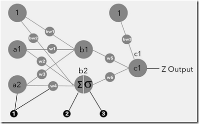
In this stage the input moves through the network to become output. To understand this stage, there are a couple of aspects that one need to understand:

  • How are the input edges collapsed in to a single value at a node ?
  • How is the input node value transformed so that it can propagate through the network?

image

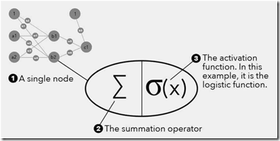
Well, specific mathematical functions are used to accomplish both the above tasks. There are two types of mathematical functions used in every node. The first is the summation operator and the second is the activation function. Every node, irrespective of whether it is a node in the hidden layer or an output node, has several inputs. These inputs have to be summed up in some way to compute the net input. These inputs are then fed in to an activation function that decides the output of the node. There are many types of activation functions- Linear, Step, Hyperbolic Tangent, Rectified Linear Unit(has become popular since 2015). The reason for using activation functions is to limit the output of a node. If you use a sigmoid function the output is generally restricted between 0 and 1. If you use a tanh function, the output is generally restricted between -1 and 1. The basic reason for using activation functions is to introduce non-linearity( Most of the real life classification problems do not have nice linear boundaries)

image

Once the basic mathematical functions are set up, it becomes obvious that any further computations would require you to organize everything in vectors and matrices. The following are the various types of vectors and matrices in a neural network

  • Weights information stored in a matrix
  • Input features stored in a vector
  • Node Inputs in a vector
  • Node outputs in a vector
  • Network error
  • Biases
Calculating the Total Error

Once the forward propagation is done and the input is transformed in to a set of nodes, the next step in the NN modeling is the computation of total error. There are several ways in which one can compute this error – Mean Squared Error , Squared Error, Root Mean Square, Sum of Square Errors

Calculation of Gradients

Why should one compute gradients, i.e. partial derivative of the error with respect to each of the weight parameter ? Well, the classic way of minimizing any function involves computing the gradient of the function with respect to some variable. In any standard multivariate calculus course, the concept of Hessian is drilled in to the students mind. If there is any function that is dependent on multiple parameters and one has to choose a set of parameters that minimizes the function, then Hessian is your friend.

Backpropagation

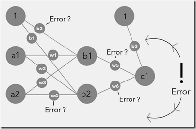
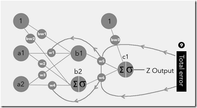
The key idea of back propagation is that one needs to update the weight parameters and one of the ways to update the weight parameters is by tweaking the weight values based on the partial derivative of the error with respect to individual weight parameters.

image

Before updating the parameter values based on partial derivatives, there is an optional step of checking whether the analytical gradient calculations are approximately accurate. This is done by a simple perturbation of weight parameter and then computing finite difference value and then comparing it with the analytical partial derivative

There are various ways to update parameters. Gradient Descent is an optimization method that helps us find the exact combination of weights for a network that will minimize the output error. The idea is that there is an error function and you need to find its minimum by computing the gradients along the path. There are three types of gradient descent methods mentioned in the book – Batch Gradient Descent method, Stochastic Gradient Descent method, Mini Batch Gradient Descent method. The method of your choice depends on the amount of data that you want to use before you want to update the weight parameters.

Constructing a Neural Network – Hand on Example

image

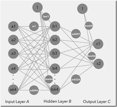
The author takes a simple example of image classification – 8 pixel by 8 pixel image to be classified as a human/chicken. For any Neural Network model, the determination of Network structure has five steps :

  • Determining Structural elements
    • Total number of input nodes: There are 64 pixel inputs
    • Total hidden layers : 1
    • Total hidden nodes : 64, a popular assumption that number of nodes in the hidden layer should be equal to the number of nodes in the input layer
    • Total output nodes: 2 – This arises from the fact that we need to classify the input in to chicken node or human node
    • Bias value : 1
    • Weight values : Random assignment to begin with
    • Learning rate : 0.5

image

  • Based on the above structure, we have 4224 weight parameters and 66 biased value weight parameters, in total 4290 parameters. Just pause and digest the scale of parameter estimation problem here.
  • Understanding the Input Layer
    • This is straightforward mapping between each pixel to an input node. In this case, the input would be gray-scale value of the respective pixel in the image
  • Understanding the Output Layer
    • Output contains two nodes carrying a value of 0 or 1.
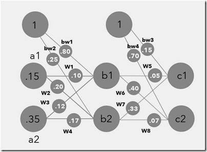
  • The author simplifies even further so that he can walk the reader through the entire process.

image

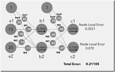
  • Once a random set of numbers are generated for each of the weight parameters, for each training sample, the output node values could be computed. Based on the output nodes, one can compute the error

image

  • Once the error has been calculated, the next step is back propagation so that the weight parameters that have been initially assigned can be updated.
  • The key ingredient of Back propagation is the computation of gradients, i.e. partial derivatives of the error with respect to various weight parameters.
  • Gradients for Output Layer weights are computed
  • Gradients for Output Layer Bias weights are computed
  • Gradients for Hidden Layer weights are computed
  • Once the gradients are computed, an optional step is to check whether numerical estimate of the gradients and the analytical value of the gradient is close enough
  • Once all the partial derivatives across all the weight parameters are computed, then the weight parameters can be updated to new values via one of the gradient adjustment methods and of course the learning rate(hyper parameter)

image

Building Neural Networks

There are many ML libraries out there such as TensorFlow, Theano, Caffe, Torch, Keras, SciKit Learn. You got to choose what works for you and go with it. TensorFlow is an open source library developed by Google that excels at numerical computation. It can be run on all kinds of computer, including smartphones and is quickly becoming a popular tool within machine learning. Tensor Flow supports deep learning( Neural nets with multiple hidden layers) as well as reinforcement learning.

TensorFlow is built on three key components:

  • Computational Graph : This defines all of the mathematical computations that will happen. It does not perform the computations and it doesn’t hold any values. This contain nodes and edges
  • Nodes : Nodes represent mathematical operations. Many of the operations are complex and happen over and over again
  • Edges represent tensors, which hold the data that is sent between the nodes.

There are a few chapter towards the end of the book that go in to explaining the usage of TensorFlow. Frankly this is an overkill for a book that aims to be an introduction. All the chapters in the book that go in to Tensor Flow coding details could have been removed as it serves no purpose. Neither does one get an decent overview of the library not does it go in to the various details.

The book is a quick read and the visuals will be sticky in one’s learning process. This book will equip you to have just enough knowledge to speak about Neural Networks and Deep Learning. Real understanding of NN and Deep NN anyways will come only from slogging through the math and trying to solve some real life problem.

book_cover

This book can be used as a companion to a more pedagogical text on survival analysis. For someone looking for an appropriate R command to use, for fitting certain kind of survival model, this book is apt. This book neither gives the intuition nor the math behind the various models. It appears like an elaborate help manual for all the packages in R, related to event history analysis.

I guess one of the reasons for the author writing this book is to highlight his package eha on CRAN. The author’s package is basically a layer on survival package that has some advanced techniques which I guess only a serious researcher in this field can appreciate. The book takes the reader through the entire gamut of models using a pretty dry format, i.e. it gives the basic form of a model, the R commands to fit the model,and some commentary on how to interpret the output. The difficulty level is not a linear function from start to end. I found some very intricate level stuff interspersed among some very elementary estimators. An abrupt discussion of Poisson regression breaks the flow in understanding Cox model and its extensions. The chapter on cox regression contains detailed and unnecessary discussion about some elementary aspects of any regression framework. Keeping these cribs aside, the book is useful as a quick reference to functions from survival, coxme, cmprsk and eha packages.

book_cover_sa_self


As the title suggests, this book is truly a self-learning text. There is minimal math in the book, even though the subject essentially is about estimating functions(survival, hazard, cumulative hazard). I think the highlight of the book is its unique layout. Each page is divided in to two parts, the left hand side of the page runs like a pitch, whereas the right hand side of the page runs like a commentary to the pitch. Every aspect of estimation and inference is explained in plain simple English. Obviously one cannot expect to learn the math behind the subject. In any case, I guess the target audience for this book comprises those who would like to understand survival analysis, run the model using some software packages and interpret the output. So, in that sense, the book is spot on. The book is 700 pages long and so all said and done, this is not a book that can be read in one or two sittings. Even thought the content is easily understood, I think it takes a while to get used the various terms, assumptions for the whole gamut of models one comes across in survival analysis. Needless to say this is a beginner’s book. If one has to understand the actual math behind the estimation and inference of various functions, then this book will equip a curious reader with a 10,000 ft. view of the subject, which in turn can be very helpful in motivating oneself to slog through the math.

Here is a document that gives a brief summary of the main chapters of the book.

cover

This book is vastly different from the books that try to warn us against incorrect statistical arguments present in media and other mundane places. Instead of targeting newspaper articles, politicians, journalists who make errors in their reasoning, the author investigates research papers, where one assumes that scientists and researchers make flawless arguments, at least from stats point of view. The author points a few statistical errors, even in the pop science book, “How to lie with statistics?”. This book takes the reader through the kind of statistics that one comes across in research papers and shows various types of flawed arguments. The flaws could arise because of several reasons such as eagerness to publish a new finding without thoroughly vetting the findings, not enough sample size, not enough statistical power in the test, inference from multiple comparisons etc. The tone of the author isn’t deprecatory. Instead he explains the errors in simple words. There is minimal math in the book and the writing makes the concepts abundantly clear even to a statistics novice. That in itself should serve as a good motivation for a wider audience to go over this 130 page book.

In the first chapter, the author introduces the basic concept of statistical significance. The basic idea of frequentist hypothesis testing is that it is dependent on p value that measure Probability(data|Hypothesis). In a way, p value measures the amount of surprise that you find in the data given that you have a specific null hypothesis in mind. If the p value turns out to be too less, then you start doubting your null and reject the null. The procedure at the outset looks perfectly logical. However one needs to keep in mind, the things that do not form a part of p value such as,

  • It does not per se measure the size of the effect.
  • Two experiments with identical data can give different p values. This is disturbing as one assumes that p value somehow knows the intention of the person doing the experiment.
  • It does not say anything about the false positive rate.

By the end of the first chapter, the author convincingly rips apart p value and makes a case for using confidence intervals. He also says that many people do not report confidence intervals because they are often embarrassingly wide and might make their effort a fruitless exercise.

The second chapter talks about statistical power, a concept that many introductory stats courses do not delve in to, appropriately. The statistical power of a study is the probability that it will distinguish an effect of a certain size from pure luck. The power depends on three factors

  • size of the bias you are looking for
  • sample size
  • measurement error

If an experiment is trying to test a subtle bias, then there needs to be far more data to even detect it. Usually the accepted power for an experiment is 80%. This means that the probability of bias detection is close to 80%. In many of the tests that have negative results, i.e the alternate is rejected, it is likely that the power of test is compromised. Why do researchers fail to take care of power in their calculations? The author guesses that it could be because the researcher’s intuitive feeling about samples is quite different from the results of power calculations. The author also ascribes to the not so straightforward math required to compute the power of study.

The problems with power also plague the other side of experimental results. Instead of detecting the true bias, the results often show inflation of true result, called M errors, where M stands for magnitude. One of the suggestions given by the author is : Instead of computing the power of a study for a certain bias detection and certain statistical significance, the researchers should instead look for power that gives narrower confidence intervals. Since there is no readily available term to describe this statistic, the author calls it assurance, which determines how often the confidence intervals must beat a specific target width. The takeaway from this chapter is that whenever you see a report of significant effect, your reaction should not be “Wow, they found something remarkable", but it needs to be, "Is the test underpowered ?". Also just because alternate was rejected doesn’t mean that alternate is absolute crap.

The third chapter talks about pseudo replication, a practice where the researcher uses the same set of patients/animals/ whatever to create repeated measurements. Instead of bigger sample sizes, the researcher creates a bigger sample size by repeated measurements. Naturally the data is not going to be independent as the original experiment might warrant. Knowing that there is a pseudo replication of the data, one must be careful while drawing inferences. The author gives some broad suggestions to address this issue

The fourth chapter is about the famous base rate fallacy where one ascribes the p value to the probability of alternate being true. Frequentist procedures that give p values merely talk about the surprise element. In no way do they actually talk about the probability of alternate treatment in a treatment control experiment. The best way to get a good estimate of probability that a result is false positive, is by considering prior estimates. The author also talks about Benjamini-Hochberg procedure, a simple yet effective procedure to control for false positive rate. I remember reading this procedure in an article by Brad Efron titled, “The future of indirect evidence”, in which Efron highlights some of the issues related to hypothesis testing in high dimensional data.

The fifth chapter talks about the often found procedure of testing two drugs with a placebo and using the results to compare the efficiency of two drugs. Various statistical errors can creep in. These are thoroughly discussed. The sixth chapter talks about double dipping, i.e. using the same data to do exploratory analysis and hypothesis testing. It is the classic case of using in-sample statistics to extrapolate out-of-sample statistics. The author talks about arbitrary stopping rules that many researchers employ for cutting short an elaborate experiment when they find statistically significant findings at the initial stage. Instead of having a mindset which says, "I might have been lucky in the initial stage", the researchers over enthusiastically stops the experiment and reports truth inflated result. The seventh chapter talks about the dangers of dichotomizing continuous data. In many research papers, there is a tendency to divide the data in to two groups and run significance tests or ANOVA based tests, thus reducing the information available from the dataset. The author gives a few examples where dichotomization can lead to grave statistical errors.

The eighth chapter talks about basic errors that one does in doing regression analysis. The errors highlighted are

  • over reliance on stepwise regression methods like forward selection or backward elimination methods
  • confusing correlation and causation
  • confounding variables and Simpson’s paradox

The last few chapters gives general guidelines to improve research efforts, one of them being “reproducible research”. 

takeawayTakeaway

Even though this book is a compilation of various statistical errors committed by researchers in various scientific fields, it can be read by anyone whose day job is data analysis and model building. In our age of data explosion, where there are far more people employed in analyzing data and who need not necessarily publish papers, this book would be useful to a wider audience. If one wants to go beyond the simple conceptual errors present in the book, one might have to seriously think about all the errors mentioned in the book and understand the math behind them.

book_cover

The book serves a nice intro to Bayes theory for an absolute newbie. There is minimal math in the book. Whatever little math that’s mentioned, is accompanied by figures and text so that a newbie to this subject “gets” the basic philosophy of Bayesian inference. The book is a short one spanning 150 odd pages that can be read in a couple of hours.  The introductory chapter of the book comprises few examples that repeat the key idea of Bayes. The author says that he has deliberately chosen this approach so that a reader does not miss the core idea of the Bayesian inference which is,

Bayesian inference is not guaranteed to provide the correct answer. Instead, it provides the probability that each of a number of alternative answers is true, and these can then be used to find the answer that is most probably true. In other words, it provides an informed guess.

In all the examples cited in the first chapter, there are two competing models. The likelihood of observing the data given each model is almost identical. So, how does one chose one of the two models ? Well, even without applying Bayes, it is abundantly obvious which of the two competing models one should go with. Bayes helps in formalizing the intuition and thus creates a framework that can be applied to situations where human intuition is misleading or vague. If you are coming from a frequentist world where “likelihood based inference” is the mantra, then Bayes appears to be merely a tweak where weighted likelihoods instead of plain vanilla likelihoods are used for inference.

The second chapter of the book gives a geometric intuition to a discrete joint distribution table. Ideally a discrete joint distribution table between observed data and different models is the perfect place to begin understanding the importance of Bayes. So, in that sense, the author provides the reader with some pictorial introduction before going ahead with numbers. 

The third chapter starts off with a joint distribution table of 200 patients tabulated according to # of symptoms and type of disease. This table is then used to introduce likelihood function, marginal probability distribution, prior probability distribution, posterior probability distribution, maximum apriori estimate . All these terms are explained using plain English and thus serves as a perfect intro to a beginner. The other aspect that this chapter makes it clear is that it is easy to obtain probability of data given a model. The inverse problem, i.e probability of model given data, is a difficult one and it is doing inference in that aspect that makes Bayesian inference powerful. 

The fourth chapter moves on to  continuous distributions. The didactic method is similar to the previous chapter. A simple coin toss example is used to introduce concepts such as continuous likelihood function,  Maximum likelihood estimate, sequential inference, uniform priors, reference priors,  bootstrapping and various loss functions.

The fifth chapter illustrates inference in a Gaussian setting and establishes connection with the well known regression framework. The sixth chapter talks about joint distributions  in a continuous setting.  Somehow I felt this chapter could have been removed from the book but I guess keeping with the author’s belief that “spaced repetition is good”, the content can be justified. The last chapter talks about Frequentist vs. Bayesian wars, i.e. there are statisticians who believe in only one of them being THE right approach. Which side one takes depends on how one views “probability” as – Is probability a property of the physical world or is it a measure of how much information an observer has about that world ? Bayesians and increasingly many practitioners in a wide variety of fields have found the latter belief to be a useful guide in doing statistical inference. More so, with the availability of software and computing power to do Bayesian inference, statisticians are latching on to Bayes like never before.

The author deserves a praise for bringing out some of the main principles of Bayesian inference using just visuals and plain English. Certainly a nice intro book that can be read by any newbie to Bayes.

book-cover


imageTakeaway :

This book is a beautiful book that describes the math behind queueing systems. One learns a ton of math tools from this book, that can be used to analyze any system that has a queueing structure within it. The author presents the material in a highly enthusiastic tone with superb clarity. Thoroughly enjoyed going through the book.

image

In the last few decades, enormous computational speed has become accessible to many. Modern day desktop has good enough memory and processing speed that enables a data analyst to compute probabilities and perform statistical inference by writing computer programs. In such a context, this book can serve as a starting point to anyone who wishes to explore the subject of computational probability. This book has 21 puzzles that can be solved via simulation.

Solving a puzzle has its own advantages. Give a dataset with one dependent variable and a set of predictors to a dozen people asking them to fit a regression model; I bet that you will see at least a dozen models, each of which could be argued as a plausible model. Puzzles are different. There are constraints put around the problem that you are forced to get that ONE RIGHT solution to the problem. In doing so, you develop much more sophisticated thinking skills.

In the introductory chapter of the book, the author provides a basic framework for computational probability by showing ways to simulate and compute probabilities. This chapter gives the reader all the ammunition required to solve the various puzzles of the book. The author provides detailed solutions that includes relevant MATLAB code, to all the 21 puzzles.

Some of my favorite puzzles from the book that are enlightening as well as paradoxical are :

  • ˆ The Gamow-Stern Elevator
  • ˆ The Pipe Smoker’s Discovery
  • ˆ A Toilet Paper Dilemma
  • ˆ Parrondo’s Paradox
  • ˆ How Long Is the Wait to Get the Potato Salad ?
  • ˆ The Appeals court Paradox

Here is the link to my document that flushes out the details of all the 21 puzzles in the book:

What’s in the above document?

I have written R code that aims to computationally solve each of the puzzles in the book. For each puzzle, there are two subsections. First subsection spells out my attempt at solving the puzzle. The second subsection contains my learning from reading through the solution given by the author. The author provides extremely detailed MATLAB code that anyone who has absolutely no exposure to MATLAB can also understand the logic. In many cases I found that the code snippets in the book looked like elaborate pseudo code. There are many good references mentioned for each of the puzzles so that interested readers can explore further aspects. In most of the cases, the reader will realize that closed form solutions are extremely tedious to derive and simulation based procedures make it easy to obtain solutions to many intractable problems.

imageimage

Every year there are at least a dozen pop math/stat books that get published. Most of them try to illustrate a variety of mathematical/statistical principles using analogies/anecdotes/stories that are easy to understand. It is a safe assumption to make that the authors of these books spend a considerable amount of time thinking about the apt analogies to use, those that are not too taxing on the reader but at the same time puts across the key idea. I tend to read at least one pop math/stat book in a year to whet my “analogy appetite”. It is one thing to write an equation about some principle and a completely different thing to be able to explain a math concept to somebody. Books such as these help in building one’s “analogy” database so that one can start seeing far more things from a math perspective. The author of this book, Jordan Ellenberg, is a math professor at University of Wisconsin-Madison and writes a math column for “Slate”. The book is about 450 odd pages and gives a ton of analogies. In this post, I will try to list down the analogies and some points made in the context of several mathematical principles illustrated in the book.

  • Survivorship bias
    • Abraham Wald’s logic of placing armor on engines that had no bullet holes
    • Mutual funds performance over a long period
    • Baltimore stockbroker parable
  • Linearity Vs. Nonlinear behavior
    • Laffer curve
  • Notion of limits in Calculus
    • Zeno’s Paradox
    • Augustin-Louis Cauchy’s and his work on summing infinite series
  • Regression
    • Will all Americans become obese? The dangers of extrapolation
    • Galton Vs. Secrist – “Regression towards mediocrity” observed in the data but both had different explanations. Secrist remained in the dark and attributed mediocrity to whatever he felt like. Secretist thought the regression he painstakingly documented was a new law of business physics, something that would bring more certainty and rigor to the scientific study of commerce. But it was just the opposite. Galton on the other hand was a mathematician and hence rightly showed that in the presence of a random effect, the regression towards mean is a necessary fact. Wherever there is a random fluctuation, one observes regression towards mean, be it mutual funds, performance of sportsmen, mood swings etc.
    • Correlation is non-transitive. Karl Pearson idea using geometry makes it easy to prove.
    • Berkson’s fallacy – Why handsome men are jerks? Why popular novels are terrible?

image

  • Law of Large numbers
    • Small school vs. Large school performance comparison
  • Partially ordered sets
    • Comparing disasters in human history
  • Hypothesis testing + “P value” + Type I error ( seeing a pattern where there is none) + Type II error(missing a pattern when there is one)
    • Experimental data from dead fish fMRI measurement: Dead fish have the ability to correctly assess the emotions the people in the pictures displayed. Insane conclusion that passes statistical tests
    • Torah dataset (304,8500 letter document) used by a group of researchers to find hidden meanings beneath the stories, genealogies and admonitions. Dangers of data mining.
    • Underpowered test : Using binoculars to detect moons around Mars
    • Overpowered test: If you study a large sample size, you are bound to reject null as your dataset will enable you to see ever-smaller effects. Just because you can detect them doesn’t mean they matter.
    • “Hot hand” in basketball : If you ask the right question, it is difficult to detect the effect statistically. The right question isn’t “Do basket players sometimes temporarily get better or worse at making shots? – the kind of yes/no question a significance test addresses. { Null – No “hothand”, Alternate : “Hot hand” } is an underpowered test . The right question is “How much does their ability vary with time, and to what extent can observers detect in real time whether a player is hot”? This is a tough question.
    • Skinner rejected the hypothesis that Shakespeare did not alliterate!
    • Null Hypothesis Significance testing, NHST,is a fuzzy version of “Proof by contradiction”
    • Testing whether a set of stars in one corner of a constellation (Taurus) is grouped together by chance?
    • Parable by Cosma Shalizi : Examining the livers of sheep to predict about future events. Very funny way to describe what’s going with the published papers in many journals
    • John Ioannidis Research paper “Why most Published Researched Findings Are False”?
    • Tests of genetic association with disease – awash with false positives
    • Example of a low powered study : Paper in Psychological science( a premier journal) concluded that “Married woman were more likely to support Mitt Romney when they were in the fertile portion of their ovulatory cycle”!
    • Low powered study is only going to be able to see a pretty big effect. But sometimes you know that the effect, if it exists, is small. In other words, a study that accurately measures the effect of a gene is likely to be rejected as statistically insignificant, while any result that passes the pvalue test is either a false positive or a true positive that massively overstates the effect
    • Uri Simonsohn, a professor at Penn brilliantly summarizes the problem of replicability as “p-hacking”(somehow getting it to the 0.05 level that enables one to publish papers)

image

    • In 2013, the association for Psychological science announced that they would start publishing a new genre of articles, called Registered Replication Reports. These reports aimed at reproducing the effects reported in widely cited studies, are treated differently from usual papers in a crucial way: The proposed experiment is accepted for publication before the study is carried out. If the outcomes support the initial finding, great news, but if not they are published anyway so that the whole community can know the full state of the evidence.
  • Utility of Randomness in math
    • “Bounded gaps” conjecture: Is there a bound for the gap between two primes? Primes get rarer and rarer as we chug along integer axis. Then what causes the gap to be bounded?
    • How many twin primes are there in the first N numbers (Among first N numbers, about N/log N are prime)?
    • Mysteries of prime numbers need new mathematical ideas that structure the concept of structurelessness itself
  • How to explain “Logarithm” to a kid? The logarithm of a positive integer can be thought as the number of digits in the positive number.
  • Forecast performance
    • Short term weather forecasts have become a possibility, given the explosion of computing power and big data. However any forecast beyond 2 weeks is dicey. On the other hand, the more data and computing power you have , some problems might yield highly accurate forecasts such as prediction of the course of an asteroid. Whatever domain you work in, you need to consider where does your domain lie between these two examples, i.e. one where big data + computing power helps and the second where big data + computing power + whatever is needed does not help you get any meaningful forecast beyond a short term forecast.
  • · Recommendation Algorithms
    • After decades of being fed with browsing data, recommendations for almost all the popular sites suck
    • Netflix prize, an example that is used by many modern Machine learning 101 courses It took 3 years of community hacking to improve the recommendation algo. Sadly the algo was not put to use by Netflix. The world moved on in three years and Netflix was streaming movies online, which makes dud recommendations less of a big deal.
  • Bayes theorem
    • Which Facebook users are likely to be involved in terrorist activities? Facebook assigns a probability that each of its users is associated with terrorist activities. The following two questions have vastly different answers. You need to be careful about what you are asking.
      1. What is the chance that a person gets put on a Facebook’s list, given that they are not a terrorist?
      2. What’s the chance that a person’s not a terrorist, given that they are on Facebook list ?
    • Why one must go Bayes? P(Data/Null) is what frequentist answers , P(Null/Data) is what a Bayesian answers
    • Are Roulette wheels biased? Use priors and experimental data to verify the same
  • Expected Value
    • Lottery ticket pricing
    • Cash WinFall : How a few groups hijacked the Massachusetts State Lottery ? Link : Boston Globe, that explains why it turned out to be a private lottery.
    • Use the additivity law of expectation to solve Buffon’s Needle problem
  • Utility curve
    • If you miss your flight, how to quantify your annoyance level?
    • Utility of dollars earned for guy moonlighting is different from that of a tenured professor
    • St Petersburg paradox
  • Error correction coding , Hamming code, Hamming distance, Shannon’s work :
    • Reducing variance of loss in Cash WinFall lottery : Choosing the random numbers with less variance is a computationally expensive problem if brute force is used. Information theory and Projective geometry could be the basis on which the successful MIT group generated random numbers that had less variance while betting.
    • Bertillion’s card system to identify criminals and Galton’s idea that redundancy in the card can be quantified, were formalized by Shannon who showed that the correlation between variables reduces the informativeness of a card
  • Condorcet Paradox
    • Deciding a three way election is riddled with many issues. There is no such thing as the public response. Electoral process defines the public response and makes peace with the many paradoxes that are inherent in deciding the public response.

Quotes from the book:

  • Knowing mathematics is like wearing a pair of X-ray specs that reveal hidden structures underneath the messy and chaotic surface of the world
  • Mathematics is the extension of common sense. Without the rigorous structure that math provides, common sense can lead you astray. Formal mathematics without common sense would turn math computations in to sterile exercise.
  • It is pretty hard to understand mathematics without doing mathematics. There is no royal road to any field of math. Getting your hands dirty is a prerequisite
  • People who go into mathematics for fame and glory don’t stay in mathematics for long
  • Just because we can assign whatever meaning we like to a string of mathematical symbols doesn’t mean we should. In math, as in life, there are good choices and there are bad ones. In the mathematical context, the good choices are the ones that settle unnecessary perplexities without creating new ones
  • We have to teach math that values precise answers but also intelligent approximation, that demands the ability to deploy existing algorithms fluently but also the horse sense to work things out on the fly that mixes rigidity with a sense of play. If we don’t do teach it that way, we are not teaching mathematics at all.
  • Field Medalist David Mumford: Dispense plane geometry entirely from the syllabus and replace it with a first course in programming.
  • “Statistically noticeable” / “Statistically detectable” is a better term than using “Statistically significant”. This should be the first statement that must be drilled in to any newbie taking stats101 course.
  • If gambling is exciting, you are doing it wrong – A powerful maxim applicable for people looking for investment opportunities too. Hot stocks provide excitement and most of the times that is all they do.
  • It is tempting to think of “very improbable” as meaning “essentially impossible”. Sadly NHST makes us infer based on “very improbable observation”. One good reason why Bayes is priceless in this aspect
  • One of the most painful aspects of teaching mathematics is seeing my students damaged by the cult of the genius. That cult tells students that it’s not worth doing math unless you’re the best at math—because those special few are the only ones whose contributions really count. We don’t treat any other subject that way. I’ve never heard a student say, "I like ‘Hamlet,’ but I don’t really belong in AP English—that child who sits in the front row knows half the plays by heart, and he started reading Shakespeare when he was 7!" Basketball players don’t quit just because one of their teammates outshines them. But I see promising young mathematicians quit every year because someone in their range of vision is "ahead" of them. And losing mathematicians isn’t the only problem. We need more math majors who don’t become mathematicians—more math-major doctors, more math-major high-school teachers, more math-major CEOs, more math-major senators. But we won’t get there until we dump the stereotype that math is worthwhile only for child geniuses

The book ends with a quote from Samuel Beckett

image

image

It was bootstrapping that made me start off on my statistics journey years ago. I have very fond memories of the days when I could understand simple things in statistics without resorting to complicating looking formulae. A few lines of code were all that was needed. Slowly I became more curious about many things in statistics and that’s how my love affair with stats began. There are two bibles that any newbie to bootstrap should go over; one by Efron & Tibshirani and the other by Davison & Hinkley. Any other specific topics, you can always understand by reading papers. It is always a nice feeling for me to read stuff about bootstrapping. However reading this book was an extremely unpleasant experience.

In the recent years with the rise of R, many authors have started writing books such as “Introduction to ____( fill in any statistical technique that you want to) using R”. With many more people adopting R, these books hope to fill the need of a data analyst who might not be willing immerse himself/herself in to the deep theories behind a technique. The target audience might want some package that can be used to crunch out numbers. Fair enough. Not everyone has the time and inclination to know the details. There are some amazing books that fill this need and do it really well. Sadly, this book is not in that category. Neither does it explains the key functions for using bootstrapping nor does it explain the code that has been sprinkled in the book. So, the R in the title is definitely a misleading one. Instead of talking about the nuances of the various functions based on author’s experience, all one gets to see is some spaghetti code in the book. I can’t imagine an author using 15 pages of the book (that too within a chapter and not the appendix) in listing various packages that have some kind of bootstrap function. That’s exactly the authors of this book have done. Insane! This book gives a historical perspective of various developments around bootstrapping techniques. You can’t learn anything specific from the book. It just gives a 10000 ft. overview of various aspects of bootstrapping. I seriously do not understand why the authors has even written this book. My only purpose in writing this review is to dissuade others from reading this book and wasting their time and money.

Introduction

The bootstrap is one of the number of techniques that are a part of a broad umbrella of nonparametric statistics that are commonly called resampling methods. It was the article by Brad Efron in 1979 that started it all. The impact of this important publication can be gauged by the following statement in Davison and Hinkley’s book :

The idea of replacing complicated and often inaccurate approximations to biases, variances and other measures of uncertainty by computer simulation caught the imagination of both theoretical researchers and users of statistical methods

Efron’s motivation was to construct a simple approximation to Jackknife procedure that was initially developed by John Tukey. Permutation methods were known since 1930s but they were ineffective beyond small samples. Efron connected bootstrapping techniques to the then available jackknife, delta method, cross validation and permutation tests. He was the first to show that bootstrapping was a real competitor to jackknife and delta method for estimating the standard error of an estimator. Throughout 1980s to 1990s, there was an explosion of papers on this subject. Bootstrap was being used for confidence intervals, hypothesis testing and more complex problems. In 1983, Efron wrote a remarkable paper that showed that bootstrap worked better than crossvalidation in classification problems of a certain kind. While these positive developments were happening, by 1990s, there were also papers that showed bootstrap estimates were not consistent in specific settings. The first published example of an inconsistent bootstrap estimate appeared in 1981. By the year 2000, there were quite a few articles that showed that bootstrapping could be a great tool to estimate various functions but it can also be inconsistent. After this brief history on bootstrapping, the chapter goes in to defining some basic terms and explaining four popular method; jackknife, delta method, cross validation and subsampling. Out of all the packages mentioned in the chapter (that take up 15 pages), I think all one needs to tinker around to understand basic principles are boot and bootstrap

Estimation

This chapter talks about improving the point estimation via bootstrapping. Historically speaking, the bootstrap method was looked at, to estimate the standard error of an estimate and later for a bias adjustment. The chapter begins with a simple example where bootstrap can be used to compute the bias of an estimator. Subsequently a detailed set of examples of using bootstrapping to improve cross validation estimate are given. These examples show that there are many instances where Bootstrapped crossvalidation technique gives a better performance than using other estimators like CV, 632 and e0 estimators. About estimating a location parameter for a random variable from a particular distribution, MLE does a great job and hence one need not really use bootstrapping. However there are cases where MLE estimates have no closed form solutions.In all such cases, one can just bootstrap away to glory. In the case of linear regression, there are two ways in which bootstrapping can be used. The first method involves residuals. Bootstrap the residuals and create a set of new dependent variables. These dependent variables can be used to form a bootstrapped sample of regression coefficients. The second method is bootstrapping pairs. It involves sampling pairs of dependent and independent variable and computing the regression coefficients. Between these two methods, the second method is found to be more robust to model misspecification.

Some of the other uses of bootstrapping mentioned in the chapter are:

  • Dealing with heteroskedastic errors by using wild bootstrap
  • Nonlinear regression
  • Non parametric regression
  • Application to CART family (bagging, boosting and random forests)

My crib about this chapter is this : You are introducing data mining techniques like LDA, QDA, bagging etc. in a chapter where the reader is supposed to get an intuition about how bootstrapping can be used to get a point estimate. Who is the target audience for this book ? A guy who is already familiar with these data mining techniques would gloss over the stuff as there is nothing new for him. A newbie would be overwhelmed by the material. For a guy who is not a newbie and who is not a data mining person, the content will be appear totally random . Extremely poor choice of content for an introductory book.

Confidence Intervals

One of the advantages of generating bootstrapped samples is that they can be used to construct confidence intervals. There are many ways to create confidence intervals. The chapter discusses bootstrap-t, iterated bootstrap, BC, BCa and tiled bootstrap. Again I don’t expect any newbie to understand clearly these methods after reading this chapter. All the author has managed to do is to give a laundry list of methods and give some description about the methods.And Yes, an extensive set of references that makes you feel that you are reading a paper and not a book. If you want to really understand these methods, the bibles mentioned at the beginning are the right sources.

Hypothesis testing

For simple examples, hypothesis testing can be done based on the confidence intervals obtained via bootstrap samples. There are subtle aspects that one needs to take care of, such as sampling from the pooled data etc. Amazing that the author doesn’t even provide some sample code to illustrate this point. The code that’s provided does sampling from individual samples. Instead code should have been provided to illustrate sampling from pooled data. Again poor choice on the way to present the content.

Time Series

The chapter gives a laundry list of bootstrap procedures in the context of time series; model based bootstrap, non overlapping block bootstrap, circular bootstrap, stationary bock bootstrap, tapered block bootstrap, dependent wild bootstrap,sieve bootstrap. Again a very cursory treatment and references to a whole lot of papers and books. The authors get it completely wrong. In an introductory book, there must be R code, there must be some simple examples to illustrate the point. Instead if you see a lot of references to papers and journal articles, the reader is going to junk this book and move on

Bootstrap variants

The same painful saga continues. The chapter gives a list of techniques – Bayesian bootstrap, Smoothed bootstrap, Parametric bootstrap, Double bootstrap, m-out-of-n bootstrap, and wild bootstrap. There is no code whatsoever to guide the reader. The explanation given to introduce these topics is totally inadequate.

When the bootstrap is inconsistent and How to remedy it ?

This chapter gives a set of scenarios when the bootstrap procedure can fail

  • For small sample sizes less than 10, bootstrapped sample is not reliable
  • Distributions that have infinite second moments
  • Estimating extreme values
  • Unstable AR processes
  • Long memory processes


imageTakeaway:

This is the worst book that I have read in the recent times. The authors are trying to cash in on the popularity of R. The title of the book is completely misleading. Neither is it an introduction to bootstrap methods nor is it an introduction to R methods for bootstrapping. All it does is give a cursory and inadequate treatment to the bootstrap technique. Do not buy or read this book. Total waste of time and money.

Next Page »