Index Funds and ETFs

 

The first three chapters of the book are targeted towards those who want to get a basic understanding of index funds. The first chapter talks about the massive growth of indexing and hence index funds & ETFs. The second chapter walks the reader through the history of various fund structures that came before index funds and ETFs. The third chapter gives a laundry list of entities that have benefited from the rise of index funds.

Chapters 4, 5 and 6 are different from the usual ETF marketing literature as they highlight the problems with index funds and ETF investing

Problems of Theory and Practice

The chapter highlights various problematic aspects of indexing

• “In the long run, stocks always go up. Hence pick an index and stay invested”. The underlying assumption is that returns earned by business are ultimately translated in to returns earned by the stock market. This is the Efficient Market Hypothesis touted by academicians. However the market has always shown cyclical behavior and the average time that supposedly long term term investor stays in any fund in 3.5 years. Given these facts, the popular philosophy of “buy and index and forget it”, looks good on paper but ultimately fails to deliver
• Risk = Reward Fallacy: The distribution of risk and fair returns is not a linear relationship. You might take on too much risk, not being aware of it, and pay for it in the long-term as markets slowly adjust price/risk anomalies, leaving you with years of unexpected under-performance.
• Markets Always Rise Fallacy – This has been debunked in many markets across many time periods
• Popular Indices are primarily Market Cap weighted, i.e. popular companies of the season make it to the index and make the index overpriced. Market cap-weighted indices will always over-represent the industries that cause a bubble in the first place. Index fund holders would always suffer the consequences of such market anomalies more than they actually deserved or even wanted.
• Lot of Capital chasing passive industry might make market overvalued
• Increased Margin Lending: To reduce operational costs, most funds are participants in the margin lending business, which in turn fuels short sellers activities
• Companies outside of index face more difficult environments: In a world where market capitalization is the key factor of stock benchmarks today, companies with a larger market capitalization experience a disproportionate flow of trading activity in their shares, making it much easier for those companies to raise fresh capital at favorable conditions through stock issuance or bond finance. Keep in mind that this quirk goes back to the issues of market cap-weighted indices. Companies not included in a specific index don’t get buying attention from countless index funds. These companies have a much harder time raising capital from markets; it’s usually at less favorable financial terms, as there is less demand for bonds or stocks issued from those companies. The rich get richer.

Problem of Participation

The author highlights some of the key pain points associated with investor participation

• Clients regularly underestimate the real fees involved even for index funds
• Clients are confused by the product variety of today’s index fund universe
• Clients have unreasonable return expectations induced by over optimistic advertising.

Another much touted wisdom is the application of asset allocation methodologies using index funds. This strategy has not delivered as expected. Target Date funds are a great example. Investors have realized that the so called “glide path” promised by the fund managers has been far from satisfactory. Most of the asset allocation strategies suggested by investment gurus is just a hogwash. The portfolio allocation – “Invest in ETFs in a specific proportion and forget it” hasn’t yielded good returns.

Problem of Narrative

The author talks about the various narratives that we hear about ETFs. He subsequently says that all those narratives never pan out. In reality, the following are the scenarios faced by index investors

• Investors don’t achieve the buy-and-hold returns advertised by fund houses
• Average holding period of a typical investor is 3.3 years
• Index fund proponents often mention the intellectual superiority of index funds and those who buy them. They are supposedly more sophisticated and advanced than investors in funds with active management, just by association. Unfortunately, there is no evidence that buyers of index funds, especially ETFs, are more sophisticated than those buying traditional mutual funds or even simple stocks. Past statistics of inflows and outflows for index funds prove that the average index fund investor behaves the same as any other ordinary mutual fund investor.
• Index investing is taking a massive bet on the market. Like any bet, it can go either ways
• Buy and Hold doctrine narrative is hardly true if one analyzes the investor behavior of ETFs and Index Funds

The last chapter of the book tries to educate the reader on the way to go about index investing. I found this chapter very pretty cliched.

Trivia from the book

• The big three index funds are Vanguard, Blackrock and StateStreet have 12 Trillion in AUM!
• World’s first investment fund was floated in 1774 by a Adriaan van Ketwich
• First index investment trust (Vanguard 500 Index Fund) was floated in 1976
• 1924 saw the birth of first two open-end mutual funds
• No one has profited more from the boom of index funds than the index originators themselves. It’s one of the best business models on the planet.
• Bogle, the godfather of index investing, ironically made his money not out of index funds
• According to SEC filings, MSCI boasts more than $1 billion in operating revenues for the year ending December 2015, operating income of over $400 million and net income of $220 million not so bad for a business that creates fictitious pools of securities in all imaginable sizes and forms. MSCI alone currently offers more than 160,000 indices.

I found nothing special about this book. May be the chapters that highlight the problems with index investing might be worth a quick read.

 

 

Machine Learning With Boosting – Summary

Gradient Boosting Algorithm is one of the powerful algos out there for solving classification and regression problems.This book gives a gentle introduction to the various aspects of the algo with out overwhelming the reader with the detailed math of the algo. The fact that there are a many visuals in the book makes the learning very sticky. Well worth a read for any one who wants to understand the intuition behind the algo.

Here is a link to a detailed summary :

Machine Learning With Boosting – Summary

 

 

 

Make Your Own Neural Network

This book is a great quick read that highlights various aspects of Neural Network components. There are three parts to the book. The first part of the book takes the reader through the various components of a Neural Network. The second part of the book equips the reader to write a simple piece of python code from scratch(not using any off-the-shelf library) that sets up a neural network, trains the neural network and test the structure for a certain set of test samples. The third part of the book adds some fun exercises that test a specific neural network.

Deep Learning as an algo and framework has become extremely popular in the last few years. In order to understand Deep Learning, a basic familiarly of Neural Networks in its original form is useful. This book acts as a good entry point for any ML newbie who wants to learn Neural Networks. Even though there are few equations mentioned in the first part of the book, the details of every component of the equation are explained in such a way that you just need to know high school math to understand the contents of the book.

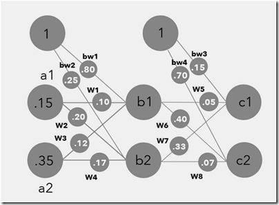
The author starts with a very simple example of estimating a conversion function that takes input in kilometers and gives the output in miles. Although you might know the exact conversion between the two scales, there is another interesting way to go about solving this problem. If you know the exact value of the input in miles, then you can guess the conversion function and then check the extent of error between the function estimate and the true value. Based on the magnitude and direction of the error, one can adjust the conversion function in such a way that the output of the function is as close to the true value as possible. The way you tweak the various parameters in the conversion function depends on the derivative of the conversion function with respect to the various parameters.

In an Neural Network retraining, one needs to compute the partial derivative of the error with respect to a weight parameter and then use that value to tweak the weight parameter. Why should one do that ? What’s partial derivative of error got to do with weight parameter updates ? One feature that is particularly explained well in the book is the fact that there is a need for delayed updates for weight parameters. If you update parameters after every training sample, then the weight parameters are going to fit only the last training sample very well and the whole model might perform badly for all the other samples. By using learning rate as a hyperparameter, one can control the amount of weight updates. The rationale for something more than linear classifier is illustrating via classifying the output of XOR operator.

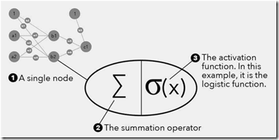
The analogy between water in a cup and activation function is very interesting. Observations suggest that neurons don’t react readily, but instead suppress the input until it has grown so large that it triggers an output. The idea of connecting the threshold with an activation function is a nice way to understand the activation functions. The idea that there are two functions that are being used on every node, one is the summation operator and the second is the activation function is illustrated via nice visuals. Even a cursory understanding of Neural Networks requires at least a basic knowledge of Matrices. The author does a great job of demonstrating the purpose of matrices, i.e. easy representation of the NN model as well as efficient computation of forward propagation and back propagation

The idea that the partial derivative is useful in tweaking the weight parameters is extremely powerful. One can visualize by thinking of a person trying to reach to the lowest point of a topsy turvy surface. There are many ways to reach the lowest point on the surface. In the process of reaching the lowest point, the gradient of the surface in several directions is essential as it will guide the person in moving in the right direction. The gradient gets smaller as you reach the minimum point. This basic calculus idea is illustrated via a set of rich visuals. Any person who has no understanding of partial derivatives will still be able to understand by going through the visuals.

The second part of the book takes the reader through a Python class that can be used to train and test a Neural Network structure. Each line of the code is explained in such a way that a Python newbie will have no problem in understanding the various components of the code.

The third part of the book invites the readers to test Neural network digit classification on a sample generated from their own handwriting. For fun, you can write down a few digits on a piece of paper and then check whether a NN network built trained based on x number of sample points can successfully recognize the digits in your handwriting.

The book shows a lot of visuals that show NN performance based on tweaking the hyperparameters such as learning rate, number of hidden layers etc. All of those visuals, I guess, will make any curious reader to explore this model further. In fact NN model in its new avatar, Deep Learning, is becoming a prerequisite skill for any Machine Learning engineer.

 

Neural Networks – A Visual Introduction For Beginners

The author says that there are five things about Neural Networks that any ML enthusiast should know:

1. Neural Networks are specific : They are always built to solve a specific problem
2. Neural Networks have three basic parts, i.e. Input Layer, Hidden Layer and Output Layer
3. Neural Networks are built in two ways
   • Feed Forward : In this type of network, signals travel only one way, from input to output. These types of networks are straightforward and used extensively in pattern recognition
   • Recurrent Neural Networks: With RNN, the signals can travel in both directions and there can be loops. Even though these are powerful, these have been less influential than feed forward networks
4. Neural Networks are either Fixed or Adaptive : The weight values in a neural network can be fixed or adaptive
5. Neural Networks use three types of datasets. Training dataset is used to adjust the weight of the neural network. Validation dataset is used to minimize overfitting problem. Testing dataset is used to gauge how accurately the network has been trained. Typically the split ratio among the three datasets is 6:2:2

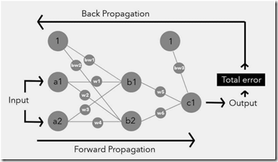
There are five stages in a Neural Network and the author creates a good set of visuals to illustrate each of the five stages:

1. Forward Propagation
2. Calculate Total Error
3. Calculate the Gradients
4. Gradient Checking
5. Updating Weights

Be it a convolution neural network(CNN) or a recurrent neural network(RNN), all these networks have a structure-or-shell that is made up of similar parts. These parts are called hyperparameters and include elements such as the number of layers, nodes and the learning rate.Hyperparameters are knobs that can tweaked to help a network successfully train. The network does not tweak these hyperparameters.

There are two types of Hyperparameters in any Neural Network, i.e. required hyperparameters and optional hyperparameters. The following are the required Hyperparameters

• Total number of input nodes. An input node contains the input of the network and this input is always numerical. If the input is not numerical, it is always converted. An input node is located within the input layer, which is the first layer of a neural network. Each input node represents a single dimension and is often called a feature.
• Total number of hidden layers. A hidden layer is a layer of nodes between the input and output layers. There can be either a single hidden layer or multiple hidden layers in a network. Multiple hidden layers means it is is a deep learning network.
• Total number of hidden nodes in each hidden layer. A hidden node is a node within the hidden layer.
• Total number of output nodes. There can be a single or multiple output nodes in a network
• Weight values. A weight is a variable that sits on an edge between nodes. The output of every node is multiplied by a weight, and summed with other weighted nodes in that layer to become the net input of a node in the following layer
• Bias values. A bias node is an extra node added to each hidden and output layer, and it connects to every node within each respective layer. The bias is a way to shift the activation function to the left or right.
• Learning Rate. It is a value that speeds up or slows down how quickly an algorithm learns. Technically this is the size of step an algo takes when moving towards global minimum

The following are the optional hyperparameters:

• Learning rate decay
• Momentum. This is the value that is used to help push a network out of local minimum
• Mini-batch size
• Weight decay
• Dropout:Dropout is a form of regularization that helps a network generalize its fittings and increase accuracy. It is often used with deep neural networks to combat overfitting, which it accomplishes by occasionally switching off one or more nodes in the network.

Forward Propagation

In this stage the input moves through the network to become output. To understand this stage, there are a couple of aspects that one need to understand:

• How are the input edges collapsed in to a single value at a node ?
• How is the input node value transformed so that it can propagate through the network?

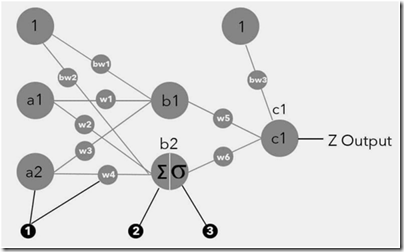
Well, specific mathematical functions are used to accomplish both the above tasks. There are two types of mathematical functions used in every node. The first is the summation operator and the second is the activation function. Every node, irrespective of whether it is a node in the hidden layer or an output node, has several inputs. These inputs have to be summed up in some way to compute the net input. These inputs are then fed in to an activation function that decides the output of the node. There are many types of activation functions- Linear, Step, Hyperbolic Tangent, Rectified Linear Unit(has become popular since 2015). The reason for using activation functions is to limit the output of a node. If you use a sigmoid function the output is generally restricted between 0 and 1. If you use a tanh function, the output is generally restricted between -1 and 1. The basic reason for using activation functions is to introduce non-linearity( Most of the real life classification problems do not have nice linear boundaries)

Once the basic mathematical functions are set up, it becomes obvious that any further computations would require you to organize everything in vectors and matrices. The following are the various types of vectors and matrices in a neural network

• Weights information stored in a matrix
• Input features stored in a vector
• Node Inputs in a vector
• Node outputs in a vector
• Network error
• Biases

Calculating the Total Error

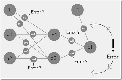
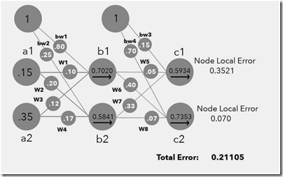
Once the forward propagation is done and the input is transformed in to a set of nodes, the next step in the NN modeling is the computation of total error. There are several ways in which one can compute this error – Mean Squared Error , Squared Error, Root Mean Square, Sum of Square Errors

Calculation of Gradients

Why should one compute gradients, i.e. partial derivative of the error with respect to each of the weight parameter ? Well, the classic way of minimizing any function involves computing the gradient of the function with respect to some variable. In any standard multivariate calculus course, the concept of Hessian is drilled in to the students mind. If there is any function that is dependent on multiple parameters and one has to choose a set of parameters that minimizes the function, then Hessian is your friend.

Backpropagation

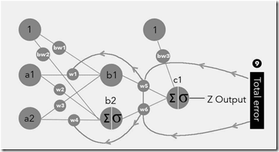
The key idea of back propagation is that one needs to update the weight parameters and one of the ways to update the weight parameters is by tweaking the weight values based on the partial derivative of the error with respect to individual weight parameters.

Before updating the parameter values based on partial derivatives, there is an optional step of checking whether the analytical gradient calculations are approximately accurate. This is done by a simple perturbation of weight parameter and then computing finite difference value and then comparing it with the analytical partial derivative

There are various ways to update parameters. Gradient Descent is an optimization method that helps us find the exact combination of weights for a network that will minimize the output error. The idea is that there is an error function and you need to find its minimum by computing the gradients along the path. There are three types of gradient descent methods mentioned in the book – Batch Gradient Descent method, Stochastic Gradient Descent method, Mini Batch Gradient Descent method. The method of your choice depends on the amount of data that you want to use before you want to update the weight parameters.

Constructing a Neural Network – Hand on Example

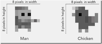
The author takes a simple example of image classification – 8 pixel by 8 pixel image to be classified as a human/chicken. For any Neural Network model, the determination of Network structure has five steps :

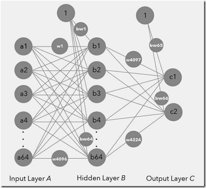
• Determining Structural elements
  • Total number of input nodes: There are 64 pixel inputs
  • Total hidden layers : 1
  • Total hidden nodes : 64, a popular assumption that number of nodes in the hidden layer should be equal to the number of nodes in the input layer
  • Total output nodes: 2 – This arises from the fact that we need to classify the input in to chicken node or human node
  • Bias value : 1
  • Weight values : Random assignment to begin with
  • Learning rate : 0.5

• Based on the above structure, we have 4224 weight parameters and 66 biased value weight parameters, in total 4290 parameters. Just pause and digest the scale of parameter estimation problem here.
• Understanding the Input Layer
  • This is straightforward mapping between each pixel to an input node. In this case, the input would be gray-scale value of the respective pixel in the image
• Understanding the Output Layer
  • Output contains two nodes carrying a value of 0 or 1.
• The author simplifies even further so that he can walk the reader through the entire process.

• Once a random set of numbers are generated for each of the weight parameters, for each training sample, the output node values could be computed. Based on the output nodes, one can compute the error

• Once the error has been calculated, the next step is back propagation so that the weight parameters that have been initially assigned can be updated.
• The key ingredient of Back propagation is the computation of gradients, i.e. partial derivatives of the error with respect to various weight parameters.
• Gradients for Output Layer weights are computed
• Gradients for Output Layer Bias weights are computed
• Gradients for Hidden Layer weights are computed
• Once the gradients are computed, an optional step is to check whether numerical estimate of the gradients and the analytical value of the gradient is close enough
• Once all the partial derivatives across all the weight parameters are computed, then the weight parameters can be updated to new values via one of the gradient adjustment methods and of course the learning rate(hyper parameter)

Building Neural Networks

There are many ML libraries out there such as TensorFlow, Theano, Caffe, Torch, Keras, SciKit Learn. You got to choose what works for you and go with it. TensorFlow is an open source library developed by Google that excels at numerical computation. It can be run on all kinds of computer, including smartphones and is quickly becoming a popular tool within machine learning. Tensor Flow supports deep learning( Neural nets with multiple hidden layers) as well as reinforcement learning.

TensorFlow is built on three key components:

• Computational Graph : This defines all of the mathematical computations that will happen. It does not perform the computations and it doesn’t hold any values. This contain nodes and edges
• Nodes : Nodes represent mathematical operations. Many of the operations are complex and happen over and over again
• Edges represent tensors, which hold the data that is sent between the nodes.

There are a few chapter towards the end of the book that go in to explaining the usage of TensorFlow. Frankly this is an overkill for a book that aims to be an introduction. All the chapters in the book that go in to Tensor Flow coding details could have been removed as it serves no purpose. Neither does one get an decent overview of the library not does it go in to the various details.

The book is a quick read and the visuals will be sticky in one’s learning process. This book will equip you to have just enough knowledge to speak about Neural Networks and Deep Learning. Real understanding of NN and Deep NN anyways will come only from slogging through the math and trying to solve some real life problem.

 

Machine Learning with Random Forests and Decision Trees

The entire book is organized as 20 small bite sized chapters. Each chapter focuses on one specific thing and explains everything via visuals(as is obvious from the title).

The author starts off by explaining the basic idea of Random Forests, i.e. a collection of decision trees that have been generated via randomization. The randomness comes from the fact that a random subset is used from training the dataset and a random set of attributes are used for splitting the data. Before understanding the

To make the understanding of random forests concrete, a simple example of classifying a set of fruits based on length, width and color is used. A decision tree for classifying fruits is drawn based on three simple attributes. This decision tree is drawn using a manual process. If the data is sufficiently scattered across various dimensions, one can use basic intuition to construct a decision tree. The result of manually drawing a decision tree is shown in various iterations. There are a few immediate takeaways from this tree, i.e. there are regions where the training data from several samples are present in the a region. This makes it difficult to conclusively say anything about the region, except in a probabilistic sense. Also there are lines in the decision space that need not necessarily be horizontal and vertical. Decision tree on the other hand only uses horizontal or vertical lines. To generate a decision tree via python, all it it takes is a few lines of code. Thanks to the massive effort behind sklearn library, there is a standardized template that one can use to build many models.

One of the disadvantages of Decision trees is the overfitting. This limitation can be obviated by the use of Random Forests. The good thing about this book is that all the data used for illustration is available on the web. One can replicate each and every figure in the book via a few lines of python code. Generating a Random Forest via sklearn is just a few lines of code. Once you have fit a Random Forest, the first thing that you might want to do is predict. There are two ways to predict the outcome of the Random Forest, one is via picking up the class that is predicted the most and the second is via obtaining class probabilities. One of the biggest disadvantages with Decision trees and Random Forest models is that they cannot be used to extrapolate.

The randomness in a random forest also comes from the fact that the number of attributes selected for splitting criteria is also random. The general rule is to pick up random set of attributes and then build a decision tree based on these randomly selected attributes. The basic idea of selecting the attributes randomly is that each decision tree is built based on a randomized set of attributes and hence there is less scope of overfitting.

One of the ways to check the validity of a model is to check its performance on a test set. Usually one employs Cross-Validation method. In the case of random forests, a better way is to use Out of Bag estimator. The basic idea of O.O.B error estimate is this: If there are N data samples and a random decision tree is drawn, on an average only 2/3rd of the data sample is used. Thus there is usually 1/3rd of the dataset that is available as test data for any tree in the random forest. Hence one can compute the accuracy of each tree and average the error of all the trees, giving rise to Out of Bag error estimate.

The author also mentions two ways in which a decision tree can be split, Gini criteria and Entropy criteria. Both these are a type of impurity measures. One of the interesting features of Random Forest algo is that it gives you the relative importance scores of various attributes. Even though they are relative measures and there are some caveats in interpreting these relative scores, overall they might be useful in certain situations.

The author ends the book with a broad set of guidelines for using Random Forest

• Use cross-validation or out of bag error to judge how good the fit is
• Better data features are the most powerful tool you have to improve your results. They trump everything else
• Use feature importances to determine where to spend your time
• Increase the number of trees until the benefit levels off
• Set the random seed before generating your Random Forest so that you get reproducible results each time
• Use a predict() or a predict_prob() where it makes sense, depending on if you want just the most likely answer, or you to know the probability of all the answers
• Investigate limiting branching either by
  • Number of splits
  • Number of data points in a branch to split
  • Number of data points in the final resulting leaves
• Investigate looking at different numbers of features for each split to find the optimum. The default number of features in many implementations of Random Forest is the square root of the number of features. However other options, such as using a percentage of the number of features, the base 2 logarithm of the number of features, or other values can be good options.

 

Decision Trees and Random Forests : A Visual Introduction For Beginners

This book provides a non-mathy entry point in to the world of decision trees and random forests.

Chapter 1 introduces the three kinds of learning algorithms:

• Supervised Learning Algorithm: The algo feeds on labeled data and then use the fitted algorithm on unlabeled data
• Unsupervised Learning Algorithm: The algo feeds on unlabeled data to figure out structure and patterns on its own
• Semi-Supervised Learning: The algo feeds on labeled and unlabeled data. The algo needs to figure out the structure and patterns of the data. However it gets some help from the labeled data.

The algorithms covered in the book fall under Supervised learning category. Before understanding the decision tree, one needs to be familiar with the basic terminology. Chapter 2 of the book goes in to the meaning of various terms such as:

• Decision Node
• Chance Node
• End Node
• Root Node
• Child Node
• Splitting
• Pruning
• Branch

Chapter 3 goes in to creating a decision tree for a trivial example using pen and paper. In the process of doing so, it touches upon various aspects of the process, i.e. splitting, determining the purity of the node, determining the class label of a node etc. All of these are subtly introduced using plain English.

Chapter 4 talks about the three main strengths and weaknesses of hand-drawn decision trees.

Three main weaknesses:

• Decision trees can change very quickly
• Decision trees can become very complex
• Decision trees can cause "paralysis by analysis"

Three main strengths:

• Decision trees force you to consider outcomes and options
• Decision trees help you visualize a problem
• Decision trees help you prioritize

Decision Trees

Chapter 5 of the book gives a list of popular Decision tree algos. Decision tree can be used to perform two tasks: Classification and Regression, the former involves classifying cases based on certain features whereas the latter involves predicting a continuous value of a target variable based on input features. The five most common decision tree algos are,

1. ID3
2. C4.5
3. C5.0
4. CHAID
5. CART

Chapter 6 of the the book goes in to showcasing a simple dataset that contains movies watched by X based on certain attributes. The objective of the algo is to predict whether X will like a movie not present in the training sample, based on certain attributes. The first step in creating decision tree involves selecting the attribute based on which the root node needs to be split. The concept of "impurity" of a node is illustrated via a nice set of visuals.

Chapter 7 goes in to the math behind splitting the node, i.e using the principles of entropy and information gain. Once a node is split, one needs a metric to measure the purity of the node. This is done via entropy. For each split of an attribute, one can compute the entropy of the subset of the nodes. To aggregate the purity measures of subsets, one needs to understand the concept of Information gain. In the context of node splitting, the information gain is computed by the difference of entropies between the parent and the weighted average entropy of the children. Again a set of rich visuals are used to explain every component in the entropy formula and information gain (Kullback-Leibler divergence).

Chapter 8 addresses common questions around Decision trees

• How/When does the algo stop splitting?
  • Allow the tree to split until every subset is pure
  • Stop the split until every leaf subset is pure
  • Adopt a stopping method
    • Stop when a tree reaches a max number of levels
    • Stop when a minimum information-gain level is reached
    • Stop when a subset contains less than a defined number of data points
• Are there other methods to measure impurity ?
  • Gini’s coefficient
• What is greedy algo ?
  • greedy algo selects nodes to build a tree by making a choice that seems best in the moment and never looks back
• What if the dataset has two identical examples ?
  • These are usually the noisy observations. Either the dataset can be increased or observations could be labeled correctly
• What if there are more than 2 classes ?
  • Logic remains the same. Only the entropy formula differs

Chapter 9 talks about the potential problems with Decision trees and the ways to address them

• Overfitting
  • Statistical significance tests can be be used to check the information gain is significant or not
  • Pruning a tree so that there nodes with sparse data or incorrect fits can be removed
• Information gain bias
  • Information Gain Ratio reduces the bias that information gain has towards attributes that have large number of subsets. It accomplishes this by taking in to consideration the size and number of branches for each attribute

Chapter 10 gives an overview of Decision Tree Algorithms. Algorithms differ in the way the following aspects are handled:

• How does the algorithm determine what to split?
• How does the algorithm measure purity?
• How does the algorithm know when to stop splitting?
• How does the algorithm prune?

Here is a list of popular Decision tree algos with their pros and cons:

• ID3 Algorithm Iterative Dichotomiser 3, is the "grandfather" of decision tree algorithms and was developed in 1986 by Ross Quinlan, a machine learning researcher.
  • Pros:
    • Easy to implement.
    • Very straightforward.
    • There is plenty of documentation available to help with implementation and working through issues.
  • Cons:
    • Susceptible to overfitting
    • Does not naturally handle numerical data.
    • Is not able to work with missing values.
• C4.5 algorithm is the successor to the ID3 algorithm and was invented in 1993 by Ross Quinlan. It makes use of many of the same elements as the ID3 but also has number of improvements and benefits.
  • Pros:
    • Can work with either a continuous or discrete dataset. This means it can be used for classification or regression and work with categorical or numerical data
    • Can work with incomplete data.
    • Solves "overfitting" by pruning and its use of the Gain Ratio.
  • Cons:
    • Constructs empty branches with zero values.
    • Tends to construct very large trees with many subsets.
    • Susceptible to overfitting.
• CART was first developed in 1984 and a unique characteristic of it is that it can only construct binary trees. ID3, C4.5 and CHAID are all able to construct multiple splits.
  • Pros:
    • Can work with either a continuous or discrete dataset. This means it can be used for classification or regression.
    • Can work with incomplete data.
  • Cons:
    • It can only split on a single variable.
    • Susceptible to instability.
    • Splitting method is biased towards nodes with more distinct values.
    • Overall, the algorithm can be biased towards nodes with more missing values.

Chapter 11 gives a sample python code to build a decision tree via CART.

Random Forests

A random forest is a machine learning algorithm that makes use of multiple decision trees to predict a result, and this collection of trees is often called an ensemble. The basic idea of random forest is that a decision tree is built based on a random set of observations from the available dataset.

Chapter 12 gives pros and cons of random forest algo

• Pros:
  • More accurate than a single decision tree
  • More stable than a single decision tree
  • Less susceptible to the negative impact of greedy search
• Cons
  • More Difficult to comprehend and interpret
  • Computationally expensive

Pros and cons of Decision tree

• Pros:
  • easier to understand and interpet
  • less computational power
• Cons:
  • tend to overfit
  • affected by small changes
  • affected by greedy search

Chapter 13 describes the basic algo behind random forest, i.e three steps. The first step involves selecting a subset of data.This is followed up by selecting random set of attributes from the bootstrapped sample.Based on the selected attributes, a best split is made and is repeated until a stopping criteria is reached.

Chapter 14 describes the way in which random forest predicts the response for a test data. There are two methods described in this chapter,i.e predicting with majority vote and predicting with mean

Chapter 15 explains the way to testing random forest for its accuracy. The method entails computing O.O.B estimate(Out of Bag error estimate).The key idea is to create a map between a data point and all the trees in which that data point does not act as a training sample. Once the map is created, for every randomized decision tree, you can find a set of data points that have not been used to train it and hence can be used to test the relevant decision tree.

Chapter 16 goes in to the details of computing attribute importance. The output of such computation is a set of relative scores for all the attributes in the dataset. These scores can be used to pre-process the data – remove all the unwanted attributes and rerun the random forest.

Chapter 17 answers some of the common questions around random forests

• How many trees go in to random forest ?
  • A safe number to start is between 64 and 128 trees
• When do I use random forest vs decision tree ?
  • If you are concerned with accuracy, go for random forest
  • If you are concerned with interpretability, go for decision tree

Chapter 18 gives a sample python code to build a random forest vis Scikit-Learn library

 

Here are some of the visuals from the book:

I think the visuals are the key takeaways from the book. You can read about the concepts mentioned in the book in a ton of places. However you might not find adequate visuals in a book that explains the math. This book is a quick read and might be worth your time as visuals serve as a power aid for learning and remembering concepts.

 

The Idiot Brain: Summary

Context

I stumbled on this book on my way to Yangon and devoured the book with in a few hours. It took me more time to write the summary than to read the book. The book is 300 pages long and full credit goes to the author for making the book so interesting.In this post, I will attempt to summarize the contents of the book.

This book is a fascinating adventure into all the aspects of the brain that are messy and chaotic. These aspects ultimately result in an illogical display of human tendencies – in the way we think, the way we feel and the way we act. The preface of the book is quite interesting too. The author profoundly apologizes to the reader on a possible scenario, i.e. one in which the reader spends a few hours on the book and realizes that it as a waste of time. Also, the author is pretty certain that some of the claims made in the book would become obsolete very quickly, given the rapid developments happening in the field of brain sciences. The main purpose of the book is to show that the human brain is fallible and imperfect despite the innumerable accomplishments that it has bestowed upon us. The book talks about some of the every day common experiences we have and ties it back to the structure of our brain and the way it functions.

Chapter 1: Mind Controls

How the brain regulates the body, and usually makes a mess of things

The human brain has evolved over several thousands of years. The brain’s function was to ensure survival of the body and hence most of the functions of the brain were akin to that of a reptile, and hence the term reptilian brain. The reptilian brain comprises Cerebellum and and the Brain Stem. However the nature and size of the human brain has undergone rapid changes in the recent past. As the nature of food consumption changed, i.e. from raw food to cooked food, the size of the brain increased,  which in turn made humans seek out more sophisticated types of food. With survival related problems having been taken care of, the human brain developed several new areas as compared to its ancestors. One of the most important developmental area is the area named neo-cortex. If one were to dissect the brain on an evolutionary time scale; the reptilian brain came first and later, the neo-cortex.

Humans have a sophisticated array of senses and neurological mechanisms. These give rise to proprioception, the ability to sense how our body is currently arranged, and which parts are going where. There is also, in our inner ear, the vestibular system that helps detect balance and position. The vestibular system and proprioception, along with the input coming from our eyes are used by the brain to distinguish between an image we see while running and a moving image seen while stationary. This interaction explains the reason we throw up during motion sickness. While sitting in a plane or a ship, there is movement, even though our body is stationary. The eyes transmit these moving signals to the brain and so does the vestibular system but the proprioreceptors do not send any signal as our body parts are stationary. This creates confusion in the brain and leads to the classic conclusion that there is poison and it has to be removed from the body. 
  

The brain’s complex and confusing control of diet and eating

Imagine we have eaten a heavy meal and our stomach is more than full, when we spot the dessert. Why do most of us ahead and gorge on the dessert? It is mainly because our brains have a disproportionate say on our appetite, and interfere in almost every food related decision. Whenever the brain sees a dessert, its pleasure pathways are activated and the brain makes an executive decision to eat the dessert and override any signals from the stomach. This is also the way protein milkshakes work. As soon as they are consumed, the dense stuff fills up the stomach, expanding it in the process and sending an artificial signal to the brain that the body is fed. Stomach expansion signals however are just one small part of diet and appetite control. They are the bottom rung of a long ladder that goes all the way up to the more complex elements of the brain. Appetite is also determined by a collection of hormones secreted by the body, some of which pull in opposite directions; the ladder therefore occasionally zigzags or even goes through loops on the way up. This explains why many people report feeling hungry less than 20 minutes after drinking a milk shake!

Why does almost every one eat between 12 and 2 pm, irrespective of the kind of work being done? One of the reasons is that the brain gets used to the pattern of eating food between those time slots and it expects food once the routine is established. This not only works for pleasant things but also for unpleasant things. Subject yourself to the pain of sitting down every day and doing some hard work like working through some technical stuff, programming, playing difficult musical notes, etc. Once you do it regularly, the brain ignores the initial pain associated with the activity making it easy to pursue such activities.

The takeaway of this section is that the brain interferes in eating and this can create problems in the way food is consumed.

The brain and complicated properties of sleep?

Why does a person need sleep? There are umpteen number of theories that have been put across. The author provides an interesting narrative of each, but subscribes to none. Instead he focuses on what exactly happens in our body that makes us sleep. The pineal gland in the brain secretes the hormone melatonin, which is involved in the regulation of circadian rhythms. The amount of secretions is inversely proportional to light signals passing through our eyes. Hence the secretions rise as day light fades and the increased secretion levels lead to feelings of relaxation and sleepiness.

This is the mechanism behind jet-lag. Travelling to another time zone means you are experiencing a completely different schedule of daylight, so you may be experiencing 11 a.m. levels of daylight when your brain thinks it’s 8 p.m. Our sleep cycles are very precisely attuned, and this throwing off of our melatonin levels disrupts them. And it’s harder to ‘catch up’ on sleep than you’d think; your brain and body are tied to the circadian rhythm, so it’s difficult to force sleep at a time when it’s not expected (although not impossible). A few days of the new light schedule and the rhythms are effectively reset.

Why do we have REM sleep? For adults, usually 20% of sleep is REM sleep and for children, 80% of sleep is REM sleep. One of the main functions of REM sleep is to reinforce, organize and maintain memories.

The brain and the fight or flight response

The thalamus can be considered the central hub of the brain. Information via the senses enters the thalamus from where it is sent to the cortex and further on to the reptilian brain. Sensory information is also sent to the amygdala, an area that is said to be the seat of EQ. If there is something wrong in the environment, even before the cortex can analyze and respond to it, the amygdala invokes the hypothalamus which in turn invokes certain types of nerve systems that generate the fight or flight response such as dilating our pupils, increasing our heart rate, shunting blood supply away from peripheral areas and directing it towards muscles etc.

  The author provides a good analogy for the thalamus system:

If the brain were a city, the thalamus would be like the main station where everything arrives before being sent to where it needs to be. If the thalamus is the station, the hypothalamus is the taxi rank outside it, taking important things into the city where they get stuff done

 

Chapter 2: Gift of memory

One hears the word "memory" thrown in a lot of places, especially among devices such as computers, laptops, mobile phones etc. Sometimes our human memory is wrongly assumed to be similar to a computer memory/ hard drive where information is neatly stored and retrieved. Far from it, our memory is extremely convoluted. This chapter talks about various intriguing and baffling properties of our brain’s memory system.

The divide between long-term and short-term memory

The way memories are formed, stored and accessed in the human brain, like everything else in the brain, is quite fascinating. Memory can be categorized into short term memory/ working memory and long term memory. Short term memory is anything that we hold in our minds for not more than a few seconds. There are tons of stuff that we think through out the day and it stays in our short term memory and then disappears. There is no physical basis for short term memories. These are associated with areas in the prefrontal cortex where they are captured as neuronal activity. Since short term memory is always in constant use, anything in the working memory is captured as neuronal activity changes very quickly and nothing persists. But then how do we have memories? This is where long term memory comes in. In fact there are a variety of long term memories.

Each of the above memories are processed and stored in various parts of the brain. The basal ganglia, structures lying deep within the brain, are involved in a wide range of processes such as emotion, reward processing, habit formation, movement and learning. They are particularly involved in co-ordinating sequences of motor activity, as would be needed when playing a musical instrument, dancing or playing basketball. The cerebellum is another area that is important for procedural memories.

An area of the brain that plays a key role in encoding the stuff that we see/hear/say/feel to memories is the hippocampus. This encodes memories and slowly moves them to the cortex where they are stored for retrieval. Episodic memories are indexed in the hippocampus and stored in the cortex for later retrieval. If everything is in some form or the other is stored in the memory, why are certain aspects more easily to recall and other difficult? This depends on the richness, repetition and intensity of the encoding. These factors will make something harder or easier to retrieve.   

The mechanisms of why we remember faces before names

I have had this problem right from undergrad days. I can remember faces very well but remembering names is a challenge. I have tough time recollecting names of colleagues, names of places that I visit, names of various clients I meet. I do find this rather painful when my mind just blanks out recalling someone’s name. The chapter gives a possible explanation – the brain’s two-tier memory system that is at work retrieving memories.

And this gives rise to a common yet infuriating sensation: recognising someone, but not being able to remember how or why, or what their name is. This happens because the brain differentiates between familiarity and recall. To clarify, familiarity (or recognition) is when you encounter someone or something and you know you’ve done so before. But beyond that, you’ve got nothing; all you can say is this person/thing is already in your memories. Recall is when you can access the original memory of how and why you know this person; recognition is just flagging up the fact that the memory exists. The brain has several ways and means to trigger a memory, but you don’t need to ‘activate’ a memory to know it’s there. You know when you try to save a file onto your computer and it says, ‘This file already exists’? It’s a bit like that. All you know is that the information is there; you can’t get at it yet.

Also visual information conveyed by the facial features of a person is far richer and sends strong signals to the brain as compared to auditory signals such as the name of a person. Short term memory is largely aural whereas long term memory relies on vision and semantic qualities. 

How alcohol can actually help you remember things

Alcohol increases release of dopamine and hence causes the brain’s pleasure pathways to get activated. This in turn creates an euphoric buzz and that’s one of the states that alcoholics seek. Alcohol also leads to memory loss. So, when does it exactly help you to remember things? Alcohol dims out the activity level of the brain and hence lessens its control on various impulses. It is like dimming the red lights on all the roads in a city. With the reduced intensity, humans tend to do many more things that they would not do while sober. Alcohol disrupts the hippocampus, the main region for memory formation and encoding. However regular alcoholics get used to a certain level of consumption. Hence any interesting gossip that an alcoholic gets to know an inebriated state, he/she is far likely to remember if his body is in an inebriated state. So, in all such situations, alcohol might actually help you remember things. The same explanation also applies to caffeine-fuelled all-nighters – take a caffeine just before the exam so that the internal state of the body is the same as the one in which the information was crammed. Once you are taking an examination in a caffeinated state, you are likely to remember stuff that you crammed in a caffeinated state. 

The ego-bias of our memory systems

This section talks about the way the brain alters memories to suit a person’s ego. It tweaks memories in such a way that it flatters the human ego and over a period of time these tweaks can become self-sustaining. This is actually very dangerous. What you retrieve from your mind changes, to flatter your ego. This means that it is definitely not a wise thing to trust your memories completely.

When and how the memory system can go wrong 

The author gives a basic list of possible medical conditions that might arise, if the memory mechanism fails in the human brain. These are

• False memories – that can be impanted in our heads by just talking
• Alzheimers – associated with significant degeneration of the brain
• Strokes can have effect on hippocampus thus leading to memory deficit
• Temporal lobe removal can cause permanent loss of long term memories
• Amnesia formed by virus attacks on hippocampus – anterograde

Chapter 3: Fear

Fear is something that comes up in a variety of shades as one ages. During childhood, it is usually fear of not meeting expectations from parents and teachers, of not fitting in a school environment etc. As one moves on to youth, it is usually the fear of not getting the right job, and fear arising out of emotional and financial insecurities. As one trudges into middle age, fears revolve around meeting the financial needs of the family, avoiding getting downsized, fear of conformity, fear of not keeping healthy etc. At each stage, we somehow manage to conquer fear by experience or live with it. However there are other kinds of fears that we carry on, through out our lives. Even though our living conditions have massively improved, our brains have not had chance to evolve. Hence there are many situations where out brains are primed to think of potential threats even when there aren’t any. You look at people who have strange phobias, people believing in conspiracy theories, having bizarre notions; all these are creations of our idiot brain.

The connection between superstition, conspiracy theories and other bizarre beliefs

Apophenia involves seeing connections where there aren’t. This to me seems to be manifestation of Type I errors in real life. The author states that it is our bias towards rejecting randomness that gives rise to superstitions, conspiracy theories etc. Since humans fundamentally find it difficult to embrace randomness, their brains cook up associations where there are none and make them hold on to the assumptions to give a sense of quasi-control in this random and chaotic world.  

Chapter 4: The baffling science of intelligence

I found this chapter very interesting as it talks about an aspect that humans are proud about, i.e. human intelligence.There are many ways in which human intelligence is manifested. But as far as tools are concerned, we have limited set of tools to measure intelligence. Whatever tools we do have do not do a good job of measurement. Take IQ for example. Did you know that average IQ for any country is 100. Yes, it is a relative scale. It means that if a deadly virus kills all the people in a country who have IQ > 100, the IQ of the country still remains 100 because it is a relative score. The Guinness Book of Records has retired the category of “Highest IQ” because of the uncertainty and ambiguity of the tests.

Charles Spearman did a great service for intelligent research in 1920’s by developing factor analysis. Spearman used a process to assess IQ tests and discovered that there was seemingly one underlying factor that underpinned test performance. This was labelled the single general factor, g, and if there’s anything in science that represents what a layman would think of as intelligence, it’s g. But even g does not equate to all intelligence. There are two types of intelligence that are generally acknowledged by the research and scientific community – fluid intelligence and crystallized intelligence. 

Fluid intelligence is the ability to use information, work with it, apply it, and so on. Solving a Rubik’s cube requires fluid intelligence, as does working out why your partner isn’t talking to you when you have no memory of doing anything wrong. In each case, the information you have is new and you have to work out what to do with it in order to arrive at an outcome that benefits you. Crystallised intelligence is the information you have stored in memory and can utilise to help you get the better of situations. It has been hypothesized that Crystallised intelligence stays stable over time but fluid intelligence atrophies as we age.

Knowledge is knowing that a tomato is a fruit; wisdom is not putting it in a fruit salad. It requires crystallised intelligence to know how a tomato is classed, and fluid intelligence to apply this information when making a fruit salad.

Some scientists believe in "Multiple Intelligence" theories where intelligence could be of varying types. Sportsmen have different kind of intelligence as compared to chess masters who have different sort of intelligence from instrument artists etc. Depending on what one chooses to spend time on, the brain develops a different kind of intelligence – just two categories (fluid and crystallized) is too restrictive to capture all types of intelligence. Even though the "Multiple Intelligence" theory appears plausible, the research community has not found solid evidence to back this hypothesis.  

Why Intelligent people often lose arguments ?

The author elaborates on Impostor syndrome, a behavior trait in intelligent people. One does not need a raft of research to believe that the more you understand something, the more you realize that you know very little about it. Intelligent people by the very way they have built up their intelligence are forever skeptical and uncertain about a lot of things. In a way their arguments seem to be balanced rather than highly opinionated. On the other hand, when you see less intelligent people, the author points out that the one can see Dunning-Kruger effect in play.

Dunning and Kruger argued that those with poor intelligence not only lack the intellectual abilities, they also lack the ability to recognise that they are bad at something. The brain’s egocentric tendencies kick in again, suppressing things that might lead to a negative opinion of oneself. But also, recognising your own limitations and the superior abilities of others is something that itself requires intelligence. Hence you get people passionately arguing with others about subjects they have no direct experience of, even if the other person has studied the subject all their life. Our brain has only our own experiences to go from, and our baseline assumptions are that everyone is like us. So if we’re an idiot…

 
Crosswords don’t actually keep your brain sharp

The author cites fMRI based research to say that intelligent brains use less brain power to think or solve through problems. While doing complex tasks, the brain activity in a set of people who are posed equi-challenging tasks showed that intelligent people could solve all the challenging tasks with out any increase in brain power. On the other hand, brain activity increased only when the task complexity increased. All these activity scans arising out prefrontal cortex scans show that it is performance that matters rather than power.  There’s a growing consensus that it’s the extent and efficiency of the connections between the regions involved (prefrontal cortex, parietal lobe and so on) that has a big influence on someone’s intelligence; the better he or she can communicate and interact, the quicker the processing and lower the effort required to make decisions and calculations. This is backed up by studies showing that the integrity and density of white matter in a person’s brain is a reliable indicator of intelligence. Having given this context, the author goes on to talk about plasticity of the brain and how musicians develop a certain aspect of motor cortex after spending years of practice.

While the brain remains relatively plastic throughout life, much of its arrangement and structure is effectively set. The long white-matter tracts and pathways will have been laid down earlier in life, when development was still under way. By the time we hit our mid-twenties, our brains are essentially fully developed, and it’s fine-tuning from thereon in. This is the current consensus anyway. As such, the general view is that fluid intelligence is ‘fixed’ in adults, and depends largely on genetic and developmental factors during our upbringing (including our parents attitudes, our social background and education). This is a pessimistic conclusion for most people, especially those who want a quick fix, an easy answer, a short-cut to enhanced mental abilities. The science of the brain doesn’t allow for such things.

To circle back to the title of the section, solving crosswords will help you become good at that task alone. Working through brain games would help you become good at that specific game alone. The brain is complex enough that just by involving in a specific activity, it does not increase all the connections across the brain and hence the conclusion that solving crosswords might make you good in that specific area but it doesn’t go anything good to the overall intelligence. Think back to those days when you knew some of your friends who could crack crossword puzzles quickly. Do a quick check on where they are now and what’s their creative output so far and judge for yourself.

The author ends the chapter by talking about one phenomenon usually commented upon – tall people perceived as being smarter than shorter people, on an average. He cites many theories and acknowledges that none are conclusive enough to validate the phenomenon.

There are many possible explanations as to why height and intelligence are linked. They all may be right, or none of them may be right. The truth, as ever, probably lies somewhere between these extremes. It’s essentially another example of the classic nature vs nurture argument.    

Chapter 5: Did you see this chapter coming ?

The information that reaches our brain via the senses is often more like a muddy trickle rather than perfect representation of the outside world. The brain then does an incredible job of creating a detailed representation of the world based on this limited information. This process itself depends on many peculiarities of an individual brain and hence errors tend to creep in. This chapter talks about the way information is reconstructed by our brains and the errors that can creep in during this process. 

Why smell is powerful than taste ?

Smell is often underrated. It is estimated that humans have a capacity to smell up to 1 trillion odours. Smell is in fact the first sense that evolves in a foetus.

There are 12 facial nerves that link the functions of the face to the brain. One of them is the Olfactory nerve. Olfactory neurons that make up the olfactory nerve are unique in many ways – these are one of the few types of neurons that can regenerate. They need to regenerate because they are directly in contact with the external world and hence atrophy. The olfactory nerve sends electrical signals to the olfactory bulb, which relays information to olfactory nucleus and piriform cortex.

In the brain, the olfactory system lies in close proximity to the limbic system and hence certain smells are strongly associated with vivid and emotional memories. This is one of the reasons why marketers carefully choose odour in display stores in order to elicit purchases from the prospects. One misconception about smell is that it can’t be fooled but research has proven that there are in fact olfactory illusions. Smell does not operate alone. Smell and taste are classed as "chemical" senses, i.e. the receptors respond to specific chemicals. There are have been experiments where subjects were unable to distinguish between two completely different food items when their olfactory senses were disabled. Think about all the days where you had a bad cold and you seem to have lost the sense of taste. The author takes a dig at wine tasters and says that all their so called abilities are a bit overrated.

How hearing and touch are related ?

Hearing and touch are linked at a fundamental level. They are both classed as mechanical senses, meaning they are activated by pressure or physical force. Hearing is based on sound, and sound is actually vibrations in the air that travel to the eardrum and cause it to vibrate.

 

The sound vibrations are transmitted to the cochlea, a spiral-shaped fluid-filled structure, and thus sound travels into our heads. The cochlea is quite ingenious, because it’s basically a long, curled-up, fluid-filled tube. Sound travels along it, but the exact layout of the cochlea and the physics of sound waves mean the frequency of the sound (measured in hertz, Hz) dictates how far along the tube the vibrations travel. Lining this tube is the organ of Corti. It’s more of a layer than a separate self-contained structure, and the organ itself is covered with hair cells, which aren’t actually hairs, but receptors, because sometimes scientists don’t think things are confusing enough on their own. These hair cells detect the vibrations in the cochlea, and fire off signals in response. But the hair cells only in certain parts of the cochlea are activated due to the specific frequencies travelling only certain distances. This means that there is essentially a frequency ‘map’ of the cochlea, with the regions at the very start of the cochlea being stimulated by higher-frequency sound waves (meaning high-pitched noises, like an excited toddler inhaling helium) whereas the very ‘end’ of the cochlea is activated by the lowest-frequency sound waves. The cochlea is innervated by the eighth cranial nerve, named the vestibulocochlear nerve. This relays specific information via signals from the hair cells in the cochlea to the auditory cortex in the brain, which is responsible for processing sound perception, in the upper region of the temporal lobe.

What about touch ?

Touch has several elements that contribute to the overall sensation. As well as physical pressure, there’s vibration and temperature, skin stretch and even pain in some circumstances, all of which have their own dedicated receptors in the skin, muscle, organ or bone. All of this is known as the somatosensory system (hence somatosensory cortex) and our whole body is innervated by the nerves that serve it.

Also touch sensitivity isn’t uniform through out the body. Like hearing, the sense of touch can also be fooled.The close connection between touch and hearing means that often if there is a problem in one, there tends to be the problem with the other.

What you didn’t know about the visual system ?

The visual system is the most dominating of all the senses and also the most complicated. If you think about the retina, only 1% of the area (fovea) can digest the finer details of the visual and the rest of the 99% of the area takes in hazy peripheral details of the visual. It is just amazing that our brain can construct the image by utilizing vast amount of peripheral detail data and make us feel that we are watching a crystal clear image. There are many aspects of visual processing mentioned in this chapter that makes you wonder at this complex mechanism that we use every day. When we move our eyes from left to right, even though we see one smooth image, the brain actually receives a series of jerky scans and it then recreates a smooth image.

 

 Visual information is mostly relayed to the visual cortex in the occipital lobe, at the back of the brain. The visual cortex itself is divided into several different layers, which are themselves often subdivided into further layers. The primary visual cortex, the first place the information from the eyes arrives in, is arranged in neat ‘columns’, like sliced bread. These columns are very sensitive to orientation, meaning they respond only to the sight of lines of a certain direction. In practical terms, this means we recognise edges. The secondary visual cortex is responsible for recognising colours, and is extra impressive because it can work out colour constancy. It goes on like this, the visual-processing areas spreading out further into the brain, and the further they spread from the primary visual cortex the more specific they get regarding what it is they process. It even crosses over into other lobes, such as the parietal lobe containing areas that process spatial awareness, to the inferior temporal lobe processing recognition of specific objects and (going back to the start) faces. We have parts of the brain that are dedicated to recognising faces, so we see them everywhere.

The author ends this section by explaining the simple mechanism by which our brain creates a 3D image from a 2D information on the retina. This mechanism is exploited by the 3D film makers to create movies for which we end up paying more money than the usual movie ticket.

Strength and Weaknesses of Human Attention

There are two questions that are relevant to the study of attention.

• What is the brain’s capacity for attention ?
•   hat is it that determines where the attention is being directed ?

Two models have been put forth for answering the first question and have been studied in various research domains. First is the Bottleneck model that says that all the information that gets in to our brains is channelled through a narrow space offered by attention. It is more like a telescope where you see a specific region but cut out all the information from other parts of the sky. Obviously this is not the complete picture in as far as our attention works. Imagine you are talking to a person in a party and somebody else mentions your name; your ears perk up and your attention darts to this somebody else and you want to know about what they are speaking about you.

To address the limitations of Bottleneck model, researchers have put forth a Capacity model that says that humans attention is finite and is available to be put to use across multiple streams of information so long as the finite resource is not exhausted. The limited capacity is said to be associated with the fact that we have limited working memory. So, can you indulge in multi-tasking without compromising on the efficiency of tasks? Not necessarily. If you have trained certain tasks to have procedural memory, then probably you can do such tasks AND do some other tasks that require conscious attention.Think about preparing a dish that you have done umpteen number of times and suddenly your brain is thinking of something completely different. So, it is possible to increase the kind of attention on a task only after committing some parts of the task to procedural memory. All this might sound very theoretical but I see this work in my music practice. Unless I build muscle memory of a raag, let us say the main piece of a raag and some of the standard phrases in a raag, there is no way I can progress to improvisations.

About the second question, most of the attention is directed to what we see. It is obvious in a way. Our eyes carry most of the signals to our brains. This is a "top-down" approach to why we pay attention. We see something and we pay attention. There is also another kind of approach – a "bottom-up", where something detected as biological significance can make us pay attention without even the conscious parts of the brain having any say on it. This makes sense as our reptilian brain needed to have paid to various stimuli before even consciously processing it.

Now, where does the idiocy of the brain come in ? There are many examples cited in the chapter, one being the "door man" experiment. The experiment is a classic reminder that when we are so tunnel focused that we sometimes miss something very apparent that’s going on in the external environment. The way I relate to this experiment is – one needs to be focused and free from distraction when one is doing a really challenging task. But at the same time, it is important to scan the environment a bit and see whether it makes sense to approach the task in the same manner that you are approaching. In other words, distancing your self from the task from time to time is the key to doing the task well. I came across a similar idea in Anne Lamott’s book – Bird by Bird. Anne Lamott mentions an incident when she almost gives up on a book, takes a break, comes back to it after a month and finishes off the book in style. Attention to a task is absolutely important but beyond a point can prove counter-productive.

Chapter 6: Personality

Historically people believed that brain had nothing to do with a person’s personality. This was until Phineas Gage case surfaced in 1850’s – Phineas Gage underwent a brain injury and subsequently his mannerisms changed completely. Since then many experiements have shown that brains do have a say in the personality. The author points out to many problems measuring the direct impact of the same on personality.

The questionable use of personality tests

Personality patterns across diverse set of individuals are difficult to infer. However there are certain aspects of personalities where we see a surprising set of common patterns. According to the Big 5 Traits theory, everyone seems to fall between two extremes of the Big 5 Traits

• Openness
• Conscientiousness
• Extrovert
• Aggreableness
• Neurotic

Now one can easily dismiss the above traits saying that they are too reductionist in nature. There are many limitations of Big 5 Theory. This theory is based on Factor Analysis, a tool that tells us the sources of variation but does not say about anything about the causation. However whether the brain evolves to suit the personality types or personalities evolve based on the brain structure is a difficult question to answer. There are many such personality tests such Type A/ Type B, Myers-Briggs Type Inventory etc. Most of these tests have been put together by amateur enthusiasts and somehow they have become popular. The author puts together a balanced account of several theories and seems to conclude that most personality tests are crap.

How anger works for you and Why it can be good thing ?

The author cites various research studies to show that anger evokes signals in the left and right brain. In the right hemisphere it produces negative, avoidance or withdrawal reactions to unpleasant things, and in the left hemisphere, positive and active behaviour. Research shows that venting anger reduces cortisol levels and relaxes the brain. Suppressing anger for a long time might cause a person to overreact to harmless situations. So, does the author advocate venting anger in every instance? Not really. All that this section does is to point out research evidence that sometimes venting out anger is ok. 

How different people find and use motivation ?

How does one get motivated to do something? This is a very broad question that will elicit a variety of answers. There are many theories and the author gives a whirlwind tour of all. The most basic of all, is that humans tend to do activities that involve pleasure and avoid those that involve pain. It is so simplistic in nature that it definitely was the first theory to be ripped apart. Then came Maslow’s theory of hierarchy which looks good on paper. The fancy pyramid of needs that every MBA student reads is something that might seem to explain motivational needs. But you can think of examples from your own life when motivation to do certain things did not neatly fit the pyramid structure. Then there is this theory of extrinsic and intrinsic motivation. Extrinsic motivations are derived from the outside world. Intrinsic motivations drive us to do things because of decisions or desires that we come up within ourselves. Some studies have shown that money can be a demotivating factor when it comes to performance. Experiments have shown that subjects without a carrot perform well and seemed to have enjoyed tasks well, as compared to subjects with a carrot. There are some other theories that talk about ego gratification as the motivating factor. Out of all the theories and quirks that have been mentioned in the chapter, the only thing that has kind of worked in my life is Zeigarnik effect, where the brain really doesn’t like things being incomplete. This explains why TV shows use cliff-hangers so often; the unresolved storyline compels people to tune into the conclusion, just to end the uncertainty. To give another example, many times I have stopped doing something when I badly wanted to work more on it. This has always been the best option in the hindsight. Work on something to an extent that you leave some of it incomplete. This gives the motivation to work on it the next day.

Chapter 7: Group Hug

Do we really need to listen to other people to understand or gauge their motives? Do facial expressions give away intentions? This is one of the questions tackled in this chapter. It was believed for a long time that the speech processing areas in the brain are Broca’s area, named for Pierre Paul Broca, at the rear of the frontal lobe,and Wernicke’s area, identified by Carl Wernicke, in the temporal lobe region. 

Damage to these areas produced profound disruptions in speech and understanding. For many years these were considered the only areas responsible for speech processing. However, brain-scanning technology has changed and since then many new developments have occurred. Broca’s area, a frontal lobe region, is still important for processing syntax and other crucial structural details, which makes sense; manipulating complex information in real-time describes much of the frontal lobe activity. Wernicke’s area, however, has been effectively demoted due to data that shows the involvement of much wider areas of the temporal lobe around it. 

via Neuroscience.com

Although the field as a whole has made tremendous progress in the past few decades, due in part to significant advances in neuroimaging and neurostimulation methods, we believe abandoning the Classic Model and the terminology of Broca’s and Wernicke’s areas would provide a catalyst for additional theoretical advancement.

Damage to Broca’s and Wernicke’s area disrupts the many connections between language-processing regions, hence aphasias. But that language-processing centres are so widely spread throughout shows language to be a fundamental function of the brain, rather than something we pick up from our surroundings. Communication, though involves non-verbal cues. Many experiments conducted on aphasia patients prove that that non-verbal cues can easily be inferred by facial expressions and thus it is difficult to fake by just talking. Your faces give away your true intentions. The basic theory behind facial expressions is that there are voluntary facial expressions and involuntary facial expressions. Poker players are excellent in controlling voluntary facial expressions and train their brains to control a certain kind of involuntary facial expressions. However we do not have full control on the involuntary facial expressions and hence an acute observer can easily spot our true intentions by paying attention to facial expressions.

The author explores situations such as romantic breakups, fan club gatherings and situations where we are predisposed to cause harm to others. The message from all these narratives is that our brain gets influenced by people around us in ways we cannot fathom completely. People around you influence the way you think and act. The aphorism – you tell me who your friends, I will tell you who you are – resonates clearly in various examples mentioned in the chapter.

Chapter 8: When the Brain breaks down

All the previous chapters in the book talk about how our brain is an idiot, when functioning in a normal way. The last chapter of the book talks about situations when the brain stops functioning in a normal way. The author explores various mental health issues such as depression, drug addiction, hallucination and nervous breakdown. The chapter does a great job of giving a gist of the competing theories out there to explain some of the mental health issues. 

Takeaway

For those whose work is mostly cerebral in nature, this book is a good reminder that we should not identify with our brains or trust our brains beyond a certain point. A healthy dose of skepticism towards whatever our brain makes us feel, think and do, is a better way to lead our lives. The book is an interesting read, with just enough good humor spread across, and with just enough scientific details. Read the book if you want to know to what extent our brains are idiosyncratic and downright stupid in their workings.

 

The Power of Habit : Summary

Most of the decisions that we take or activities that we do, on a daily basis are not a result of deliberate thought. These are the result of habits that we have built over time. We realize some of these decisions/activities as habits but often carry out many activities in auto-pilot mode. This is good as it frees our mind to do other things. The flip side is that we do not seem to be in control of the actions and hence feel powerless.

This book by Charles Duhigg goes in to various details about habit, i.e. how do habits arise ? what are the triggers to our habits ? why is it difficult to change some of our habits ? what should be done to change our habits. In this post, I will try to briefly summarize the contents of the book.

The Habit Loop

The author explains the basic framework of any habit formation via what he calls,"The Habit Loop". In order to explain this framework, the reader is taken through a few specific cases that triggered an active research in this area. There have been many recent pop-science books that have mentioned H.M, a unique patient in the medical case history. What’s unique about H.M is that his hippocampus was removed surgically to avoid frequent convulsions. This created a testbed for several experiments relating to memory as H.M forgot anything he learnt in a few seconds.

The author mentions one such patient,Eugene Pauly, whose medical condition has led to an explosion of habit formation research. Eugene Pauly like H.M could not remember any new learnings beyond a few seconds. His ability to store anything new was severely damaged. However there was one thing peculiar about him. He was able to do certain activities effortlessly. The activities that were outcomes of past habits were all intact. In fact the most surprising aspect of this patient that eventually lead to a ton of research is that, Eugene Pauly was able to learn new habits, despite not being able to commit anything to memory. Dr. Larry Squire was the first person to study Eugene Pauly and report his findings in a medical journal. Larry Squire found that there are similar neurological processes for habit formulation across all individuals and the part of the brain that plays a major role in it is Basal Ganglia.

A series of experiments that were done on rats showed that habit formation has a specific pattern. When one is learning a new activity, there is a spike in neurological activity in the brain. However once the brain learns something, the basal ganglia takes over and there is a decrease in the brain activity. Also, it is not the case that the entire activity is in auto-pilot. The author explains the three-step habit loop as follows

• First, there is a cue, a trigger that tells your brain to go into automatic mode and which habit to use. The cues fall in to one of the five categories; time, location, emotional state, other people, immediately preceding action.
• Second, there is a routine, which can be physical or mental or emotional pattern
• Third, there is a reward which helps your brain figure out if this particular loop is worth remembering for the future.

Over time, this loop – cue, routine reward – becomes more and more automatic. The cue and reward become intertwined until a powerful sense of anticipation and craving emerges. Eventually a habit is born.Another finding that emerged from experiments on Eugene Pauly is that a minor tweak in the components of the habit loop can completely wreck the habit. This means a few aspects can wreck our good habits that have been painfully cultivated. It also means that bad habits can be changed by tweaking the habit loop.

The takeaway from this chapter is that one needs to be aware of the habit loop in many of the activities that we perform in our daily life. It is estimated that 40% of the decisions that we take and activities that we do are based on habits. It is very likely that some of the decisions on a daily basis might be sub-optimal. It is also likely that some of the activities/habits that we carry need to change. By realizing the cue, routine and reward components of our activities, we can develop self-awareness that will go a long way in empowering us to create a change.

The Craving Brain

The author speaks about "craving", an important ancillary component in the habit loop, that makes the loop in to a habit. If one reflects about cue-routine-reward loop for a few minutes, it becomes clear that there must be someother element that makes us go over the cue-routine-reward path. Something that powers the habit loop should be present in order to inculcate a new habit/ change an existing habit. That something is a craving for the reward.

Wolfram Schultz, a Cambridge scientist, in a series of experiments with monkeys, observed that there was a spike in monkey’s brain activity much before the reward was given. This led to an hypothesis that there is some sort of craving feeling that gets activated as soon as one sees a cue. This craving is the one that powers the habit loop. The author uses a few examples from the marketing world such as Febreze and Pepsodent to strengthen the "craving" hypothesis. In the hindsight, if you think about it for sometime, you can easily get convinced by looking a few situations in your own life where a cue created a craving that made you go through a specific routine to obtain the reward.

The Golden Rule of Habit Change

The author shares a motley collection of stories to illustrate two other aspects of habit loop. Stories about the success of Alcoholics Anonymous, Bucs(NFL) team performance, Mandy(a normal looking girl who has an obsessive tendency to bite her nails till they bled) illustrate a method to break bad habits. In all these stories, a common theme that runs is: the awareness of the cue and reward made it possible for the routine to be tweaked to obtain the same cue and reward with a healthy routine. All the above stories seem to end in a happy state by identifying the cue, identifying the actual reward and then tweaking the routine. However the habits break down under stress. Alumni of AA seemed to fall in to bad habits once tested at their limits and so is the case with other stories. The author then talks about a critical component of sustaining the habit loop – Belief, i.e one’s belief in the possibility of change.

One might read the first three chapters and cast aside the whole content as common sense. Possible. However if you reflect about the various activities that you do in your daily life and analyze whether every activity is a carefully well thought out deliberate action or not?. My guess is most of us will realize that the so called actions that we perform, be it at work or at home, are habits that we have acquired over time. Some bad, Some good. We might feel powerless to change bad habits. However the framework suggested in the first three chapters of the book offers a way to experiment with our lives and see if we could make a meaningful change in our habits.

Key stone Habits

Is there a pecking order among the various habit loops in our life? Is there any specific type of habit that has a disproportionate effect on our lives? The author calls such habits as key stone habits that can transform our lives. Keystone habits say that success doesn’t depend on getting every single thing right, but instead relies on identifying a few key priorities and fashioning them into powerful levers.In order to support his thesis, the author gives the following examples:

1. Paul O’Neill focused on one key stone habit "safety" and changed the entire culture of Alcoa.
2. Bob Bowman targeted a few specific habits that had nothing to do with swimming and everything to do with creating right mindset. He coached Phelps and we all know the rest of the story. We need to get a few small wins and they can create massive transformation
3. American Library Association’s Task Force on Gay Liberation decided to focus on one modest goal: convincing the Library of Congress to reclassify books about the gay liberation. It succeeded. It was a small win and eventually created a cascade of big wins

Key stone habits encourage change and subsequently can create a unique culture in an organization. The author gives various examples that show that a conscious effort in sustaining the culture can result in massive positive outcomes.

One of the takeaways of this chapter is the importance of journaling. If you want to pay attention to what you eat and control diet, food journaling has been found very useful. In a similar, journaling about anything that you want to change/improve can help you identify the components of habit loops. Self awareness is half the battle won.

Starbucks and the Habit of Success

Starbucks is an unique place for many reasons. One of the reasons is that it employs many youngsters just out of college. These young recruits, in all likelihood, would not have faced angry customers before and hence they find it difficult to fit in to the professional setting. Credit goes to Starbucks for teaching life skills to thousands of recruits. The way Starbucks accomplishes this is worth knowing and this chapter goes in to some of the details. At the core of all the education that Starbucks imparts is all-important habit: Will power

The company spent millions of dollars developing curriculums to train employees on self-discipline. Executives wrote workbooks that, in effect, serve as guides to how to make willpower a habit in workers’ lives. Those curriculums are, in part, why Starbucks has grown from a sleepy Seattle company into a behemoth with more than seventeen thousand stores and revenues of more than $10 billion a year.

It is not an easy task to bring about self-discipline in a massive organization. What Starbucks did is a great lesson for anyone who wants to master self-discipline. Starbucks realized that their employees tendency to self-discipline themselves depended on the way they handled themselves at few inflection points. Hence it was a organization wide practice where employees would write/talk/share about their intended behavior, much before the inflection points.

In a way this is like an entrepreneur writing in his journal about potential inflection points in his/her startup’s future journey and then gearing up for an appropriate response. Institutionalizing this kind of response among its vast workforce is what has made Starbucks sustain its profitability year after year.

The takeaway from this chapter is that one should always consider that willpower is a finite resource and spend it appropriately over a day so that we get to maintain a healthy dose of self-discipline in our lives.

What Target knows much before you do

The author uses examples from the marketing world to drive home the point that if you dress a new something in old habits, it’s easier for the public to accept it. The takeaway from this chapter is a well known message is that it pays to monitor your customers habits closely.

The last few chapters of the book talks about habit formation in societies.

Here’s a visual from the web that captures the essence of the book

Takeaway

Habit is a choice that we deliberately make at some point, and then stop thinking about it, but continue doing, often every day. The book delves in to the basic components of habit formation loop. The book might take a few hours to read but is well worth the time as it makes the reader conscious of his/her habit loops. Once you recognize a habit loop, you seem to be much more control of your habits and hence your choices.

 

Graph Databases : Book Summary

Neo4j’s founder Emil Eifrem shares a bit of history about the way Neo4j was started. Way back in 1999, his team realized that the database that was being internally used had a lot of connections between discrete data elements. Like many successful companies which grow out of a founder’s frustration with status quo, Neo4j began its life from the founding team’s frustration with the fundamental problem with the design of relational databases. The team started experimenting on various data models centered around graphs. Much to their dismay, they found no readily available graph database to store their connected data. Thus began the team’s journey in to building a graph database from scratch. Project Neo was born. What’s behind the name Neo4j ? The 4 in Neo4j does not stand for version number. All the versions numbers are appended after the word Neo4j. I found one folksy explanation on stackoverflow that goes like this,   

The Neo series of databases was developed in Sweden and attracted the ‘j’ suffix with the release of version 4 of the graph database. The ‘j’ is from the word ‘jätteträd’, literally "giant tree", and was used to indicate the huge data structures that could now be stored.

Incidentally the ‘neo’ portion of the name is a nod to a Swedish pop artist Linus Ingelsbo, who goes by the name NEO. In Neo1 the example graph was singers and bands and featured the favourite artists of the developers, including NEO. This was changed to the movie data set in the version 4 release.

There are other people speculating that Neo refers to "The Matrix" character Neo, fighting the "relational tables". It was recently announced that Neo4j would be called Neo5j as a part of latest branding exercise. In one of the recent blog post from the company, it was said that j in Neo4j stood for Java as the original graph database was writtein as a java library.

Preface

This talks about the purpose of the book, i.e to introduce graphs and graph databases to technology practitioners, including developers, database professionals, and technology decision makers. It also explains the main changes in the content of this book as compared to the first edition. The changes are mainly in the areas of Cypher syntax and modeling guidelines.

Introduction

A graph is nothing but a collection of edges and vertices. Having said that, there are many different ways in which the graph can be stored. One of the most popular form of graph model is the labeled property graph, which is characterized as

• It contains nodes and relationships
• Node contain properties(key-value pairs)
• Nodes can be labeled with one or more labels
• Relationships are names and directed, and always have a start and end node
• Relationships can also contain properties

Rough Classification

Given the plethora of products in this space, it is better to have some sort of binning. The chapter bins the products in to two groups.

1. Technologies used primarily for transactional online graph persistence, typically accessed directly in real time from an application
2. Technologies used primarily for offline graph analytics, typically performed as a series of batch steps

Broader Classification

The chapter also says that one of the other ways to slice the graph space is via graph data models, i.e. property graph, RDF triples and hypergraphs. In the appendix for the book, there is a much broader classification given for the NOSQL family of products. I will summarize the contents of appendix in this section as I found the appendix very well written.

Rise of NOSQL:

The NOSQL movement has mainly arisen because of 3 V’s

• Volume of data : There has been a deluge of semi-structured data in the recent decade and storing it all in an structured relational data format has been fraught with difficulties. Storing connections gives rise to complicated join queries for CRUD operations.
• Velocity of data read and writes and schema changes
• Variety of data

Relational databases are known to provide ACID transactions; Atomic, Consistent, Isolated, Durable. NOSQL databases instead have BASE properties; Basic availability, Soft-state, Eventual consistency. Basic availability means that the data store appears to work most of the time. Soft-state stores don’t have to be write-consistent, nor do replicas have to be mutually consistent all the time. Eventual consistency stores exhibit consistency at some later point.

Types of NOSQL Databases:

NOSQL databases can be divided in to 4 types, i.e.

• Document Stores :Document databases store and retrieve documents, just like an electronic filing cabinet. These stores act like a key-value pair with some sort of indexing in place for quicker retrieval. Since the data model is one of disconnected entities, stores tend to scale horizontally. Also writes are atomic at a document level. Technology has not matured for writes across multiple documents. MongoDB and CouchDB are two examples of Document stores.
• Key-Value Stores :Key-value stores are cousins of the document store family, but their lineage comes from Amazon’s Dynamo database. They act like large, distributed hashmap data structures that store and retrieve opaque values by key. A client stores a data element by hashing a domain-specific key. The hash function is crafted such that it provides a uniform distribution across the available buckets, thereby ensuring that no single machine becomes a hotspot. Given the hashed key, the client can use that address to store the value in a corresponding bucket. These stores are similar to document stores but offer a higher level of insight in to the data stores. Riak-for instance- also offers visibility into certain types of structured data. In any case, these stores are optimized for high availability and scale.Riak and Redis are two example of Key-Value stores.
• Column Family : These stores are modeled on Google’s BigTable. The data model is based on sparsely populated table whose rows can contain arbitrary columns, the keys which provide natural indexing. The four building blocks of Column family databasestore are column, super column, column family and super column family. HBase is an example of Column-oriented database.
• Graph Databases : All the three previous types of databases are still aggregate stores. Querying them for insight into data at scale requires processing by some external application infrastructure. Aggregate stores are not built to deal with highly connected data This is where Graph databases step in. A graph database is an online, operational database management with CRUD methods that expose a graph model. Graph databases are generally built for use with transactional systems.There are two properties that are useful to understand while investigating graph technologies  
  • The underlying storage: Some graph databases use "native graph storage", which is optimized and designed for storing and managing graphs.Not all graph database technologies use native graph storage. Some serialize the graph data in to relational database,OOPS database etc
  • Processing engine : Some graph databases are capable of index-free adjacency, i.e. nodes point to each other in the database. For graphs that use index-free processing, the authors use the term "native graph processing"

  Besides adopting a specific approach to storage and processing, Graph databases also adopt a specific model. There are various models such as property graphs, hypergraphs and triples. Hypergraphs are mainly useful for representing many-to-many relationships. Triple stores typically provide SPARQL capabilities to reason about and store RDF data. Triple stores generally do not support index-free adjacency and are not optimized for storing property graphs. To perform graph queries, triple stores must create connected structures from independent facts, which adds latency to each query. Hence the sweet sport for a triple store is analytics, where latency is a secondary consideration, rather than OLTP.  

Power of Graph Databases:

The power of graph databases lies in performance, agility and flexibility. Performance comes from the fact that search can be localized to a portion of graph. Flexibility comes from the fact that there is little impedance between the way business communicates the requirements and the way the graph is modeled. Agility comes from the fact that graph databases are schema less and hence all the new connections can easily be accommodated.

Options for Storing Connected Data

This chapter takes a simple example of modeling friends and friend of friends relations via a RDBMS. SQL code is given to extract a few basic questions an user might have, while looking at a social graph. The queries, even for simple questions, become very complex. It quickly becomes obvious to anyone reading this chapter that modeling connections via RDMBS is challenging, for the following reasons:

• Join tables add accidental complexity
• Foreign key constraints add additional development and maintenance overhead
• Sparse tables with nullable columns require special checking in code
• Several expensive joins are needed to discover nested relationships
• Reverse queries are difficult to execute as the SQL code becomes extremely complicated to write and maintain

NOSQL databases are also not scalable for storing connected data. By the very nature of document stores/key-value stores/ columnar family, the lack of connection or relation as a first class object makes it difficult to achieve scale. Even though there is some sort of indexing available in most of the NOSQL databases, they do not have index free adjacency feature. This implies that there is a latency in querying connected data.

The chapter ends with showcasing a graph database to store connections and it is abundantly clear by this point in the chapter that, by giving relationship the status of first class object, graph databases make it extremely easy to represent and maintain connected data. Unlike RDBMS and NOSQL stores in which connected data necessitates developers to write data processing logic in the application layer, graph databases offer a convenient and a powerful alternative.

Data Modeling with Graphs

The path from a real life representation of data to a data model in the graph database world is short. In fact one can use almost the same lingo to talk about various aspects while referring to graph data. This is unlike the RDBMS world where one needs to translate the real life representation to a logical model via "normalization-denormalization" route. In the latter world, there is a semantic dissonance between conceptualization of a model and database’s instantiation of that model

The chapter begins by introducing Cypher, an expressive graph database query language. Cypher is designed to be easily read and understood by developers, database professionals, and business stakeholders. Its ease of use derives from the fact that it is in accord with the way we intuitively describe graphs using diagrams. Cypher is composed of clauses like most other query languages. The chapter introduces some of the main clauses such as MATCH, RETURN, WHERE, CREATE, MERGE, DELETE, SET, FOREACH, UNION, WITH, START.

There are two examples used in the chapter that serve to show the contrast in the steps involved in modeling data in the relational world and graph world. In the relational world, one takes the white-board model, creates an ER diagram, and then a normalized representation of the model and finally a denormalized form. Creating a normalized representation involves incorporating foreign key relationships to avoid redundancy. Once the database model has been adapted to a specific domain, there is an additional denormalization work that needs to be done so as to suit the database and not the user. This entire sequence of steps creates an impedance between real life representation and the data base representation. One of the justifications given to this effort expended is that it is one time investment and it will payoff as the data grows. Sadly, given that data has 3V’s in the current age, i.e. Volume, Velocity and Variety, this argument no longer holds good. It is often seen that RDBMS data models undergo migrations with changing data structures. What once seemed to be a solid top-down robust approach falls apart quickly. In the graph world, the effort put in translating a white-board model in to a database model is minimal, i.e. what you sketch on a keyboard is what you store in the database. These two examples mentioned illustrate the fact that conceptual to implementation dissonance is is far less for graph database than an RDBMS.

The chapter also gives some guidelines in creating graphs so that they match up the BASE properties of NOSQL databases. By the end of the chapter, a reader ends up getting a good understanding of Cypher query language. If one is a complete newbie to Neo4j, it might be better to take a pause here and experiment with Cypher before going ahead with the rest of the book.

Building a Graph Database application

The basic guidelines for data modeling are

• Use nodes to represent entities – that is, the things in our domain that are interesting to us
• Use relations to represent relations between entities and to establish a semantic context for each entity
• Use relationship direction to further clarify relationship semantics. Many relationships are asymmetric and hence it makes sense to always represent a relation with a certain direction
• Use node attributes to represent entity attributes, plus any entity meta-data
• Use relationship attributes to represent the strength, weight, quality of the relationship etc.
• While modeling a node, make sure that it does not connect two nodes
• It is always better to represent both a fine grained and a coarse grained relationship between two nodes. This helps in quickly querying at a coarse grained level.
• The key idea of using graph as a way to model the data is that one can do an iterative model for creating nodes and relationships

Application Architecture

There are two ways in which Neo4j can be used in an application. One is the embedded-server mode and the rest is REST API mode.

Clustering

All writes to Neo4j can be written to the master or a slave. This capability at an application level is an extremely powerful feature. These kind of powerful features are not present in other graph databases.

Load Balancing

There is no native load balancing available in Neo4j. However it is up to the network infra to create load balancing. One needs to introduce a network level rebalancer to separate out the read and write queries. Infact Neo4j exposes an API call to indicate whether the server is a master or slave.

Since cache partitioning is an NP Hard problem, one can use a technique called "cache-sharding" to route the query to that specific server that has a highest probability of finding a cache to serve the query. The way to route and cache queries is dependent on the domain in which the graph database is being developed.

Testing

If you need to debug any function written in any language, one needs sample input. In the case of testing graph, one needs to create a small graph of a few dozen nodes and relationships, so that this localized graph can be used to check any anomalies in the graph model. It is always better to write a lot of simple tests checking various parts of the graph than relying on one single universal test for the entire graph. As the graph evolves, an entire set of regression framework of tests can be formulated.

Importing and Bulk Loading Data

Most of the deployments of any kind of database requires some sort of content to be imported in to the database. This section of the chapter talks about importing data from a csv format. The headers in the csv file should be specified in such a way that they reflect whether the pertinent columns is an ID/LABEL/TYPE/property. Once the csv files are in the relevant format, they can be imported via neo4j-import command. One can also do a batch import via Cypher queries using LOAD CSV. In my line of work, I deal with a lot of RDF input files and there is an open source stored procedure that one can use to import any large RDF in to Neo4j.

Usually doing a bulk import of any file should be preceded by index creation process. Indexes will make lookups faster during and after the load process. Creating indexes on any type of is quite straightforward via Cypher commands. If the indexing is only helpful during data loading process, one can delete the index after the bulk data load is completed. For large datasets, it is suggested that one uses PERIODIC COMMIT command so that the transactions are committed only after a certain set of rows have been processed.

Graphs in the Real World

Why Organizations choose Graph Databases ?

Some of the reasons that organizations choose graph databases are :

• "Minutes to Millisecond" performance requirement – Using an index free adjacency, a graph database turns complex joins into fast graph traversals, thereby maintaining millisecond performance irrespective of the overall size of the dataset
• Drastically accelerated development cycles : Graph model reduces the impedance mismatch between the technical and the business domains
• Extreme business responsiveness- Schema-free nature of the graph database coupled with the ability to simultaneously relate data elements in lots of different ways allows a graph database solution evolve as the business needs evolve.
• Enterprise ready -The technology must be robust, scalable and transactional. There are graph databases in the market that provide all the -ilities, i.e transactionability, high-availability, horizontal read scalability and storage of billions of triples

 Common Use cases

  The chapter mentions the following as some of the most common usecases in the graph database world:

1. Social Networks Modeling
2. Recommendations (Inductive and Suggestive)
3. Geospatial data
4. Master Data Management
5. Network and Data Center Management
6. Authorization and Access Control

Graphs in the real world

There are three usecases that are covered in detail. Reading through these usecases gives one a good introduction of various types of data modeling aspects including writing good cypher queries. Reading through the Cypher queries pre-supposes that the reader is slightly comfortable with Cypher. To get the best learning out of these examples, it is better to write out the Cypher queries before looking at the constructed queries. One gets an immediate feedback about the way to construct efficient Cypher queries.

Graph Database Internals

This chapter gives a detailed description of Neo4j graph database internals.

Native Graph Processing

A Graph database has native processing capabilities if it exhibits a property called index-free adjacency. A database engine that utilizes index-free-adjacency is one that maintains direct reference to its adjacent nodes. This enables the query times to be independent of the graph size.

A nonnative graph database uses global indexes to link nodes. These indexes add a layer of indirection to each traversal, thereby incurring computational costs. To traverse a network of m steps, the cost of indexed approach is O(m log n) whereas the cost is O(m) for an implementation that uses index-adjacency. To create a index-free adjacency in graphs, it is important to create an architecture that supports this property. Neo4j has painfully built this over a decade and one can see their efforts by querying a large graph. In my work, I have worked with pure triple stores and some sort of global indexing built on the triple stores. The performance of Neo4j is zillion times better than the databases that I have worked on. Hence a big fan of Neo4j.

Native Graph Storage

Neo4j stores data in a number of different file formats. There are separate data files for nodes, relationships and properties. Node store is a fixed size record store.Each node record is 9 bytes in length. The Node ID is created in such a way that node lookup is O(1) instead of O(log n). The constituents of the node record are 1) ID of the first relationship, 2) ID of the first property 3) label store of the node. Relationships are also stored in fixed length records whose constituents are 1) start Node ID 2) end Node ID 3) pointer to the previous relationship and pointer to the next relationship.

With fixed-sized records, traversals are implemented simply by chasing the pointers around a datastructure. The basic idea of searching in a Neo4j boils down to locating the first record in the relationship chain and then chasing various pointers. Apart from this structure, Neo4j also has a caching feature that makes increases its performance.

Programmatic APIs

Neo4j exposes four types of API for a developer and they are

1. Kernel API
2. Core API
3. Traverser API

The Core API allows developers to fine-tune their queries so that they exhibit high affinity with the underlying graph. A well-written Core API query is often faster than any other approach. The downside is that such queries can be verbose, requiring considerable developer effort. Moreover, their high affinity with the underlying graph makes them tightly coupled to its structure. When the graph structure changes, they can often break. Cypher can be more tolerant of structural changes things such as variable-length paths help mitigate variation and change. The Traversal Framework is both more loosely coupled than the Core API (because it allows the developer to declare informational goals), and less verbose, and as a result a query written using the Traversal Framework typically requires less developer effort than the equivalent written using the Core API. Because it is a general-purpose framework, however, the Traversal Framework tends to perform marginally less well than a well-written Core API query

Nonfunctional characteristics

Evaluation

One of the ways to evaluate the performance of database is via 1) the number of transactions that can be handled in an ACID way and 2) the number of read and write queries that can be processed on a database.

Transactions are semantically identical to traditional database transactions. Writes occur with in the same transaction context, with write locks being taken for consistency purposes on any nodes and relationships involved in the transaction. The following talks about the way transaction is implemented

The transaction implementation in Neo4j is conceptually straightforward. Each transaction is represented as an in-memory object whose state represents writes to the database. This object is supported by a lock manager, which applies write locks to nodes and relationships as they are created, updated, and deleted. On transaction rollback, the transaction object is discarded and the write locks released, whereas on successful completion the transaction is committed to disk.

Scale

For a platform like Neo4j, one cannot talk of scale based on # of transactions per second. One needs to think about scale along atleast three different axis.

• Capacity: The current release of Neo4j can support single graphs having tens of billions of nodes, relationships, and properties.The Neo4j team has publicly expressed the intention to support 100B+ nodes/relationships/properties in a single graph as part of its road map
• Latency: The architecture of Neo4j makes the performance almost constant irrespective of the size of the graph. Most queries follow a pattern whereby an index is used to find a starting node and the remainder is pointer chasing. Performance does not depend on the size of the graph but depends on the data being queried.
• Throughput: Neo4j has a constant time performance irrespective of the graph size. We might think that extensive read writes will make the performance of the entire database to go down. However one sees that the typical read, write queries happen on a localized graph and hence there is scope to optimize at an application level.

Holy grail of scalability

The future goal of most graph databases is to be able to partition a graph across multiple machines without application-level intervention, so that read and write access to the graph can be scaled horizontally. In the general case this is known to be an NP Hard problem, and thus impractical to solve.

Predictive Analysis with Graph Theory

The chapter starts off with a basic description of depth-first and breadth-first graph traversal mechanisms. Most useful algorithms aren’t pure breadth-first but are informed to some extent. Breadth-first search underpins numerous classical graph algorithms, including Dijkstra’s algorithm. The last chapter talks about several graph theoretical concepts that can be used to analyze Networks.

Takeaway

The book gives a good introduction to various aspects of any generic graph database, even though most of the contents are Neo4j specific. This book is 200 pages long but it packs so much content in it that one needs to read slowly to understand thorughly various aspects of a graph databases. If you have been exposed to native triple stores,then this book will be massively useful to get an idea about Neo4j’s implementation of property-graph model – an architecture that makes all the CRUD operations on a graph database very efficient.

 

Learning Cypher : Summary

Cypher is a query language for Neo4j graph database. The basic model in Neo4j can be described as

• Each node can have a number of relationships with other nodes
• Each relationship goes from one node either to another node or to the same node
• Both nodes and relationships can have properties, and each property has a name and a value

Cypher was first introduced in Nov 2013 and since then the popularity of graph databases as a category has taken off. The following visual shows the pivotal moment:

Looking at the popularity of Cypher, Neo4j was made open source in October 2015. Neo4j founders claim that the rationale behind the decision was that a common query syntax could be followed across all the graph databases. Cypher provides a declarative syntax, which is readable and powerful and a rich set of graph patterns can be recognized in a graph.

Via Neo4j’s blog:

Cypher is the closest thing to drawing on a white board with a keyboard. Graph databases are whiteboard friendly; Cypher makes them keyboard friendly.

Given that Cypher has become open source and has the potential to become the de facto standard in graph database segment, it becomes important for anyone working with graph data to have a familiarity with the syntax. Since the syntax looks like SQL syntax, has some pythonic element to the query formulation, it can be easily picked up by reading a few articles on it. Do you really need a book for it ? Not necessarily. Having said that, this book reads like a long tutorial and is not dense. It might be worth one’s time to read this book to get a nice tour of various aspects of Cypher.

Chapter 1 : Querying Neo4j effectively with Pattern Matching

Querying a graph database using API is usually very tedious. I have had this experience first hand while working on a graph database that had ONLY API interface to obtain graph data. SPARQL is a relief in such situations but SPARQL has a learning curve. I would not call it steep, but the syntax is a little different and one needs to get used to thinking in triples, for writing effective SPARQL queries. Writing effective SPARQL queries entails thinking in subject-predicate-object terms. Cypher on the other hand is a declarative query language, i.e. it focuses on the aspects of the result rather than on methods or ways to get the result. Also it is human-readable and expressive

The first part of the chapter starts with instructions to set up a new Neo4j instance. Neo4j server can be run as a standalone machine with the client making API calls OR can be run as an embedded component in an application. For learning purpose, working with standalone server is the most convenient option as you have a ready console to test out sample queries. The second part of the chapter introduces a few key elements of Cypher such as

• MATCH
• RETURN
• () for nodes
• [] for relations
• -> for directions
• – for choosing bidirectional relations
• Filtering matches via specifying node labels and properties
• Filtering relationships via specifying relationship labels and properties
• OPTIONAL to match optional paths
• Assigning the entire paths to a variable
• Passing parameters to Cypher queries
• Using built in functions such as allShortestPaths
• Matching paths that connect nodes via a variable number of hops

Chapter 2 : Filter, Aggregate and Combine Results

This chapter introduces several Cypher statements that can be used to extract summary statistics of various nodes and relationships in a graph. The following are the Cypher keywords explained in this chapter

• WHERE for text and value comparisons
• IN to filter based on certain values
• "item identifier IN collection WHERE rule" pattern that can be used to work with collections. This pattern is similar to list comprehension in python
• LIMIT and SKIP for pagination purposes. The examples do not use ORDER BY which is crucial for obtaining paginated results
• SORT
• COALESCE function to work around null values
• COUNT(*) and COUNT(property value) – Subtle difference between the two is highlighted
• math functions like MIN, MAX, AVG
• COLLECT to gather all the values of properties in a certain path pattern
• CASE WHEN ELSE pattern for conditional expressions
• WITH to separate query parts
• UNION and UNION ALL

Chapter 3 : Manipulating the Database

This chapter talks about Create, Update and Delete operations on various nodes and relations. The Cypher keywords explained in the chapter are

• CREATE used to create nodes, relationships and paths
• CREATE UNIQUE
• SET for changing properties and labels
• MERGE to check for an existing pattern and create the pattern if it does not exist in the database
• MERGE SET and MERGE CREATE for setting properties during merge operations
• REMOVE for removing properties and labels
• DELETE
• FOREACH pattern to loop through nodes in a path

By the end of this chapter, any reader should be fairly comfortable in executing CRUD queries. The queries comprise three phases

1. READ : This is the phase where you read data from the graph using MATCH, OPTIONAL, and MATCH clauses
2. WRITE : This is the phase where you modify the graph using CREATE, MERGE, SET and all other clauses
3. RETURN : This is the phase where you choose what to return to the caller

Improving Performance

This chapter mentions the following guidelines for creating queries in Neo4j :

• Use Parametrized queries: Wherever possible, write queries with parameters that allows engine to reuse the execution of the query. This takes advantage of the fact the Neo4j engine can cache the query
• Avoid unnecessary clauses such as DISTINCT based on the background information of the graph data
• Use direction wherever possible in match clauses
• Use a specific depth value while searching for varying length paths
• Profile queries so that the server does not get inundated by inefficient query construction
• Whenever there is large number of nodes belonging to a certain label, it is better to create index. In fact while importing a large RDF it is always better to create indices on certain types of nodes.
• Use constraints if you are worried about property redundancy

Chapter 4 :  Migrating from SQL

The chapter talks about various tasks involved in migrating data from a RDBMS to a graph database. There are three main tasks in migrating from SQL to a graph data base :

1. Migrating the schema from RDBMS to Neo4j
2. Migrating the data from tables to Neo4j
3. Migrating queries to let your application continue working

It is better to start with an ER diagram that is close to the white-board representation of the data. Since graph databases can closely represent a white-board than the Table structure mess(primary key, foreign key, cardinality), one can quickly figure out the nodes and relationships needed for the graph data. For migrating the actual data, one needs to import the data in to relevant CSV and load the CSV in to Neo4j. The structure of various CSV files to be generated depends on the labels, nodes, relationships of the graph database schema. Migrating queries from RDMBS world in to graph database world is far more easier as Cypher is a declarative syntax. It is far quicker to code the various business requirement queries using Cypher syntax.

Chapter 5 : Operators and Functions

The last section of the book contains a laundry list of operators and functions that one can use in creating a Cypher query. It is more like a cheat sheet but with elaborate explanation of various Cypher keywords

Takeaway

This book gives a quick introduction to all the relevant keywords needed to construct a Cypher query. In fact it is fair to describe the contents of the book as a long tutorial with sections and subsections that can quickly bring a Cypher novice up to speed.