Machine Learning With Boosting – Summary

Gradient Boosting Algorithm is one of the powerful algos out there for solving classification and regression problems.This book gives a gentle introduction to the various aspects of the algo with out overwhelming the reader with the detailed math of the algo. The fact that there are a many visuals in the book makes the learning very sticky. Well worth a read for any one who wants to understand the intuition behind the algo.

Here is a link to a detailed summary :

Machine Learning With Boosting – Summary

 

 

 

Make Your Own Neural Network

This book is a great quick read that highlights various aspects of Neural Network components. There are three parts to the book. The first part of the book takes the reader through the various components of a Neural Network. The second part of the book equips the reader to write a simple piece of python code from scratch(not using any off-the-shelf library) that sets up a neural network, trains the neural network and test the structure for a certain set of test samples. The third part of the book adds some fun exercises that test a specific neural network.

Deep Learning as an algo and framework has become extremely popular in the last few years. In order to understand Deep Learning, a basic familiarly of Neural Networks in its original form is useful. This book acts as a good entry point for any ML newbie who wants to learn Neural Networks. Even though there are few equations mentioned in the first part of the book, the details of every component of the equation are explained in such a way that you just need to know high school math to understand the contents of the book.

The author starts with a very simple example of estimating a conversion function that takes input in kilometers and gives the output in miles. Although you might know the exact conversion between the two scales, there is another interesting way to go about solving this problem. If you know the exact value of the input in miles, then you can guess the conversion function and then check the extent of error between the function estimate and the true value. Based on the magnitude and direction of the error, one can adjust the conversion function in such a way that the output of the function is as close to the true value as possible. The way you tweak the various parameters in the conversion function depends on the derivative of the conversion function with respect to the various parameters.

In an Neural Network retraining, one needs to compute the partial derivative of the error with respect to a weight parameter and then use that value to tweak the weight parameter. Why should one do that ? What’s partial derivative of error got to do with weight parameter updates ? One feature that is particularly explained well in the book is the fact that there is a need for delayed updates for weight parameters. If you update parameters after every training sample, then the weight parameters are going to fit only the last training sample very well and the whole model might perform badly for all the other samples. By using learning rate as a hyperparameter, one can control the amount of weight updates. The rationale for something more than linear classifier is illustrating via classifying the output of XOR operator.

The analogy between water in a cup and activation function is very interesting. Observations suggest that neurons don’t react readily, but instead suppress the input until it has grown so large that it triggers an output. The idea of connecting the threshold with an activation function is a nice way to understand the activation functions. The idea that there are two functions that are being used on every node, one is the summation operator and the second is the activation function is illustrated via nice visuals. Even a cursory understanding of Neural Networks requires at least a basic knowledge of Matrices. The author does a great job of demonstrating the purpose of matrices, i.e. easy representation of the NN model as well as efficient computation of forward propagation and back propagation

The idea that the partial derivative is useful in tweaking the weight parameters is extremely powerful. One can visualize by thinking of a person trying to reach to the lowest point of a topsy turvy surface. There are many ways to reach the lowest point on the surface. In the process of reaching the lowest point, the gradient of the surface in several directions is essential as it will guide the person in moving in the right direction. The gradient gets smaller as you reach the minimum point. This basic calculus idea is illustrated via a set of rich visuals. Any person who has no understanding of partial derivatives will still be able to understand by going through the visuals.

The second part of the book takes the reader through a Python class that can be used to train and test a Neural Network structure. Each line of the code is explained in such a way that a Python newbie will have no problem in understanding the various components of the code.

The third part of the book invites the readers to test Neural network digit classification on a sample generated from their own handwriting. For fun, you can write down a few digits on a piece of paper and then check whether a NN network built trained based on x number of sample points can successfully recognize the digits in your handwriting.

The book shows a lot of visuals that show NN performance based on tweaking the hyperparameters such as learning rate, number of hidden layers etc. All of those visuals, I guess, will make any curious reader to explore this model further. In fact NN model in its new avatar, Deep Learning, is becoming a prerequisite skill for any Machine Learning engineer.

 

Neural Networks – A Visual Introduction For Beginners

The author says that there are five things about Neural Networks that any ML enthusiast should know:

1. Neural Networks are specific : They are always built to solve a specific problem
2. Neural Networks have three basic parts, i.e. Input Layer, Hidden Layer and Output Layer
3. Neural Networks are built in two ways
   • Feed Forward : In this type of network, signals travel only one way, from input to output. These types of networks are straightforward and used extensively in pattern recognition
   • Recurrent Neural Networks: With RNN, the signals can travel in both directions and there can be loops. Even though these are powerful, these have been less influential than feed forward networks
4. Neural Networks are either Fixed or Adaptive : The weight values in a neural network can be fixed or adaptive
5. Neural Networks use three types of datasets. Training dataset is used to adjust the weight of the neural network. Validation dataset is used to minimize overfitting problem. Testing dataset is used to gauge how accurately the network has been trained. Typically the split ratio among the three datasets is 6:2:2

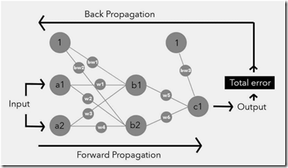
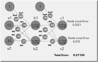
There are five stages in a Neural Network and the author creates a good set of visuals to illustrate each of the five stages:

1. Forward Propagation
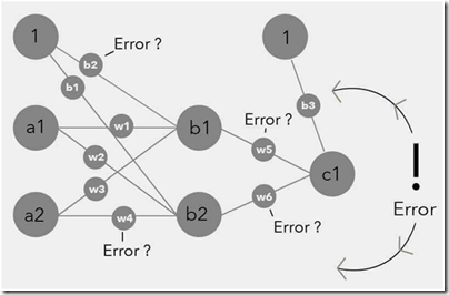
2. Calculate Total Error
3. Calculate the Gradients
4. Gradient Checking
5. Updating Weights

Be it a convolution neural network(CNN) or a recurrent neural network(RNN), all these networks have a structure-or-shell that is made up of similar parts. These parts are called hyperparameters and include elements such as the number of layers, nodes and the learning rate.Hyperparameters are knobs that can tweaked to help a network successfully train. The network does not tweak these hyperparameters.

There are two types of Hyperparameters in any Neural Network, i.e. required hyperparameters and optional hyperparameters. The following are the required Hyperparameters

• Total number of input nodes. An input node contains the input of the network and this input is always numerical. If the input is not numerical, it is always converted. An input node is located within the input layer, which is the first layer of a neural network. Each input node represents a single dimension and is often called a feature.
• Total number of hidden layers. A hidden layer is a layer of nodes between the input and output layers. There can be either a single hidden layer or multiple hidden layers in a network. Multiple hidden layers means it is is a deep learning network.
• Total number of hidden nodes in each hidden layer. A hidden node is a node within the hidden layer.
• Total number of output nodes. There can be a single or multiple output nodes in a network
• Weight values. A weight is a variable that sits on an edge between nodes. The output of every node is multiplied by a weight, and summed with other weighted nodes in that layer to become the net input of a node in the following layer
• Bias values. A bias node is an extra node added to each hidden and output layer, and it connects to every node within each respective layer. The bias is a way to shift the activation function to the left or right.
• Learning Rate. It is a value that speeds up or slows down how quickly an algorithm learns. Technically this is the size of step an algo takes when moving towards global minimum

The following are the optional hyperparameters:

• Learning rate decay
• Momentum. This is the value that is used to help push a network out of local minimum
• Mini-batch size
• Weight decay
• Dropout:Dropout is a form of regularization that helps a network generalize its fittings and increase accuracy. It is often used with deep neural networks to combat overfitting, which it accomplishes by occasionally switching off one or more nodes in the network.

Forward Propagation

In this stage the input moves through the network to become output. To understand this stage, there are a couple of aspects that one need to understand:

• How are the input edges collapsed in to a single value at a node ?
• How is the input node value transformed so that it can propagate through the network?

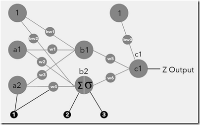
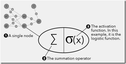
Well, specific mathematical functions are used to accomplish both the above tasks. There are two types of mathematical functions used in every node. The first is the summation operator and the second is the activation function. Every node, irrespective of whether it is a node in the hidden layer or an output node, has several inputs. These inputs have to be summed up in some way to compute the net input. These inputs are then fed in to an activation function that decides the output of the node. There are many types of activation functions- Linear, Step, Hyperbolic Tangent, Rectified Linear Unit(has become popular since 2015). The reason for using activation functions is to limit the output of a node. If you use a sigmoid function the output is generally restricted between 0 and 1. If you use a tanh function, the output is generally restricted between -1 and 1. The basic reason for using activation functions is to introduce non-linearity( Most of the real life classification problems do not have nice linear boundaries)

Once the basic mathematical functions are set up, it becomes obvious that any further computations would require you to organize everything in vectors and matrices. The following are the various types of vectors and matrices in a neural network

• Weights information stored in a matrix
• Input features stored in a vector
• Node Inputs in a vector
• Node outputs in a vector
• Network error
• Biases

Calculating the Total Error

Once the forward propagation is done and the input is transformed in to a set of nodes, the next step in the NN modeling is the computation of total error. There are several ways in which one can compute this error – Mean Squared Error , Squared Error, Root Mean Square, Sum of Square Errors

Calculation of Gradients

Why should one compute gradients, i.e. partial derivative of the error with respect to each of the weight parameter ? Well, the classic way of minimizing any function involves computing the gradient of the function with respect to some variable. In any standard multivariate calculus course, the concept of Hessian is drilled in to the students mind. If there is any function that is dependent on multiple parameters and one has to choose a set of parameters that minimizes the function, then Hessian is your friend.

Backpropagation

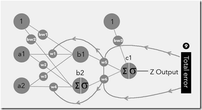
The key idea of back propagation is that one needs to update the weight parameters and one of the ways to update the weight parameters is by tweaking the weight values based on the partial derivative of the error with respect to individual weight parameters.

Before updating the parameter values based on partial derivatives, there is an optional step of checking whether the analytical gradient calculations are approximately accurate. This is done by a simple perturbation of weight parameter and then computing finite difference value and then comparing it with the analytical partial derivative

There are various ways to update parameters. Gradient Descent is an optimization method that helps us find the exact combination of weights for a network that will minimize the output error. The idea is that there is an error function and you need to find its minimum by computing the gradients along the path. There are three types of gradient descent methods mentioned in the book – Batch Gradient Descent method, Stochastic Gradient Descent method, Mini Batch Gradient Descent method. The method of your choice depends on the amount of data that you want to use before you want to update the weight parameters.

Constructing a Neural Network – Hand on Example

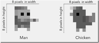
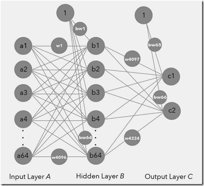
The author takes a simple example of image classification – 8 pixel by 8 pixel image to be classified as a human/chicken. For any Neural Network model, the determination of Network structure has five steps :

• Determining Structural elements
  • Total number of input nodes: There are 64 pixel inputs
  • Total hidden layers : 1
  • Total hidden nodes : 64, a popular assumption that number of nodes in the hidden layer should be equal to the number of nodes in the input layer
  • Total output nodes: 2 – This arises from the fact that we need to classify the input in to chicken node or human node
  • Bias value : 1
  • Weight values : Random assignment to begin with
  • Learning rate : 0.5

• Based on the above structure, we have 4224 weight parameters and 66 biased value weight parameters, in total 4290 parameters. Just pause and digest the scale of parameter estimation problem here.
• Understanding the Input Layer
  • This is straightforward mapping between each pixel to an input node. In this case, the input would be gray-scale value of the respective pixel in the image
• Understanding the Output Layer
  • Output contains two nodes carrying a value of 0 or 1.
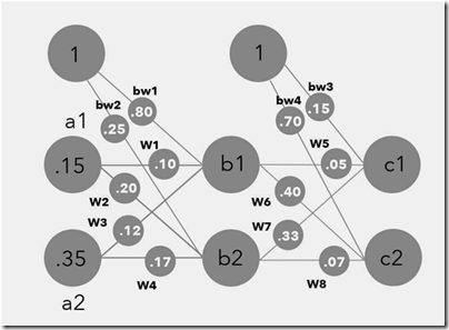
• The author simplifies even further so that he can walk the reader through the entire process.

• Once a random set of numbers are generated for each of the weight parameters, for each training sample, the output node values could be computed. Based on the output nodes, one can compute the error

• Once the error has been calculated, the next step is back propagation so that the weight parameters that have been initially assigned can be updated.
• The key ingredient of Back propagation is the computation of gradients, i.e. partial derivatives of the error with respect to various weight parameters.
• Gradients for Output Layer weights are computed
• Gradients for Output Layer Bias weights are computed
• Gradients for Hidden Layer weights are computed
• Once the gradients are computed, an optional step is to check whether numerical estimate of the gradients and the analytical value of the gradient is close enough
• Once all the partial derivatives across all the weight parameters are computed, then the weight parameters can be updated to new values via one of the gradient adjustment methods and of course the learning rate(hyper parameter)

Building Neural Networks

There are many ML libraries out there such as TensorFlow, Theano, Caffe, Torch, Keras, SciKit Learn. You got to choose what works for you and go with it. TensorFlow is an open source library developed by Google that excels at numerical computation. It can be run on all kinds of computer, including smartphones and is quickly becoming a popular tool within machine learning. Tensor Flow supports deep learning( Neural nets with multiple hidden layers) as well as reinforcement learning.

TensorFlow is built on three key components:

• Computational Graph : This defines all of the mathematical computations that will happen. It does not perform the computations and it doesn’t hold any values. This contain nodes and edges
• Nodes : Nodes represent mathematical operations. Many of the operations are complex and happen over and over again
• Edges represent tensors, which hold the data that is sent between the nodes.

There are a few chapter towards the end of the book that go in to explaining the usage of TensorFlow. Frankly this is an overkill for a book that aims to be an introduction. All the chapters in the book that go in to Tensor Flow coding details could have been removed as it serves no purpose. Neither does one get an decent overview of the library not does it go in to the various details.

The book is a quick read and the visuals will be sticky in one’s learning process. This book will equip you to have just enough knowledge to speak about Neural Networks and Deep Learning. Real understanding of NN and Deep NN anyways will come only from slogging through the math and trying to solve some real life problem.