Machine Learning With Boosting – Summary

Gradient Boosting Algorithm is one of the powerful algos out there for solving classification and regression problems.This book gives a gentle introduction to the various aspects of the algo with out overwhelming the reader with the detailed math of the algo. The fact that there are a many visuals in the book makes the learning very sticky. Well worth a read for any one who wants to understand the intuition behind the algo.

Here is a link to a detailed summary :

Machine Learning With Boosting – Summary

 

 

 

Make Your Own Neural Network

This book is a great quick read that highlights various aspects of Neural Network components. There are three parts to the book. The first part of the book takes the reader through the various components of a Neural Network. The second part of the book equips the reader to write a simple piece of python code from scratch(not using any off-the-shelf library) that sets up a neural network, trains the neural network and test the structure for a certain set of test samples. The third part of the book adds some fun exercises that test a specific neural network.

Deep Learning as an algo and framework has become extremely popular in the last few years. In order to understand Deep Learning, a basic familiarly of Neural Networks in its original form is useful. This book acts as a good entry point for any ML newbie who wants to learn Neural Networks. Even though there are few equations mentioned in the first part of the book, the details of every component of the equation are explained in such a way that you just need to know high school math to understand the contents of the book.

The author starts with a very simple example of estimating a conversion function that takes input in kilometers and gives the output in miles. Although you might know the exact conversion between the two scales, there is another interesting way to go about solving this problem. If you know the exact value of the input in miles, then you can guess the conversion function and then check the extent of error between the function estimate and the true value. Based on the magnitude and direction of the error, one can adjust the conversion function in such a way that the output of the function is as close to the true value as possible. The way you tweak the various parameters in the conversion function depends on the derivative of the conversion function with respect to the various parameters.

In an Neural Network retraining, one needs to compute the partial derivative of the error with respect to a weight parameter and then use that value to tweak the weight parameter. Why should one do that ? What’s partial derivative of error got to do with weight parameter updates ? One feature that is particularly explained well in the book is the fact that there is a need for delayed updates for weight parameters. If you update parameters after every training sample, then the weight parameters are going to fit only the last training sample very well and the whole model might perform badly for all the other samples. By using learning rate as a hyperparameter, one can control the amount of weight updates. The rationale for something more than linear classifier is illustrating via classifying the output of XOR operator.

The analogy between water in a cup and activation function is very interesting. Observations suggest that neurons don’t react readily, but instead suppress the input until it has grown so large that it triggers an output. The idea of connecting the threshold with an activation function is a nice way to understand the activation functions. The idea that there are two functions that are being used on every node, one is the summation operator and the second is the activation function is illustrated via nice visuals. Even a cursory understanding of Neural Networks requires at least a basic knowledge of Matrices. The author does a great job of demonstrating the purpose of matrices, i.e. easy representation of the NN model as well as efficient computation of forward propagation and back propagation

The idea that the partial derivative is useful in tweaking the weight parameters is extremely powerful. One can visualize by thinking of a person trying to reach to the lowest point of a topsy turvy surface. There are many ways to reach the lowest point on the surface. In the process of reaching the lowest point, the gradient of the surface in several directions is essential as it will guide the person in moving in the right direction. The gradient gets smaller as you reach the minimum point. This basic calculus idea is illustrated via a set of rich visuals. Any person who has no understanding of partial derivatives will still be able to understand by going through the visuals.

The second part of the book takes the reader through a Python class that can be used to train and test a Neural Network structure. Each line of the code is explained in such a way that a Python newbie will have no problem in understanding the various components of the code.

The third part of the book invites the readers to test Neural network digit classification on a sample generated from their own handwriting. For fun, you can write down a few digits on a piece of paper and then check whether a NN network built trained based on x number of sample points can successfully recognize the digits in your handwriting.

The book shows a lot of visuals that show NN performance based on tweaking the hyperparameters such as learning rate, number of hidden layers etc. All of those visuals, I guess, will make any curious reader to explore this model further. In fact NN model in its new avatar, Deep Learning, is becoming a prerequisite skill for any Machine Learning engineer.

 

Neural Networks – A Visual Introduction For Beginners

The author says that there are five things about Neural Networks that any ML enthusiast should know:

1. Neural Networks are specific : They are always built to solve a specific problem
2. Neural Networks have three basic parts, i.e. Input Layer, Hidden Layer and Output Layer
3. Neural Networks are built in two ways
   • Feed Forward : In this type of network, signals travel only one way, from input to output. These types of networks are straightforward and used extensively in pattern recognition
   • Recurrent Neural Networks: With RNN, the signals can travel in both directions and there can be loops. Even though these are powerful, these have been less influential than feed forward networks
4. Neural Networks are either Fixed or Adaptive : The weight values in a neural network can be fixed or adaptive
5. Neural Networks use three types of datasets. Training dataset is used to adjust the weight of the neural network. Validation dataset is used to minimize overfitting problem. Testing dataset is used to gauge how accurately the network has been trained. Typically the split ratio among the three datasets is 6:2:2

There are five stages in a Neural Network and the author creates a good set of visuals to illustrate each of the five stages:

1. Forward Propagation
2. Calculate Total Error
3. Calculate the Gradients
4. Gradient Checking
5. Updating Weights

Be it a convolution neural network(CNN) or a recurrent neural network(RNN), all these networks have a structure-or-shell that is made up of similar parts. These parts are called hyperparameters and include elements such as the number of layers, nodes and the learning rate.Hyperparameters are knobs that can tweaked to help a network successfully train. The network does not tweak these hyperparameters.

There are two types of Hyperparameters in any Neural Network, i.e. required hyperparameters and optional hyperparameters. The following are the required Hyperparameters

• Total number of input nodes. An input node contains the input of the network and this input is always numerical. If the input is not numerical, it is always converted. An input node is located within the input layer, which is the first layer of a neural network. Each input node represents a single dimension and is often called a feature.
• Total number of hidden layers. A hidden layer is a layer of nodes between the input and output layers. There can be either a single hidden layer or multiple hidden layers in a network. Multiple hidden layers means it is is a deep learning network.
• Total number of hidden nodes in each hidden layer. A hidden node is a node within the hidden layer.
• Total number of output nodes. There can be a single or multiple output nodes in a network
• Weight values. A weight is a variable that sits on an edge between nodes. The output of every node is multiplied by a weight, and summed with other weighted nodes in that layer to become the net input of a node in the following layer
• Bias values. A bias node is an extra node added to each hidden and output layer, and it connects to every node within each respective layer. The bias is a way to shift the activation function to the left or right.
• Learning Rate. It is a value that speeds up or slows down how quickly an algorithm learns. Technically this is the size of step an algo takes when moving towards global minimum

The following are the optional hyperparameters:

• Learning rate decay
• Momentum. This is the value that is used to help push a network out of local minimum
• Mini-batch size
• Weight decay
• Dropout:Dropout is a form of regularization that helps a network generalize its fittings and increase accuracy. It is often used with deep neural networks to combat overfitting, which it accomplishes by occasionally switching off one or more nodes in the network.

Forward Propagation

In this stage the input moves through the network to become output. To understand this stage, there are a couple of aspects that one need to understand:

• How are the input edges collapsed in to a single value at a node ?
• How is the input node value transformed so that it can propagate through the network?

Well, specific mathematical functions are used to accomplish both the above tasks. There are two types of mathematical functions used in every node. The first is the summation operator and the second is the activation function. Every node, irrespective of whether it is a node in the hidden layer or an output node, has several inputs. These inputs have to be summed up in some way to compute the net input. These inputs are then fed in to an activation function that decides the output of the node. There are many types of activation functions- Linear, Step, Hyperbolic Tangent, Rectified Linear Unit(has become popular since 2015). The reason for using activation functions is to limit the output of a node. If you use a sigmoid function the output is generally restricted between 0 and 1. If you use a tanh function, the output is generally restricted between -1 and 1. The basic reason for using activation functions is to introduce non-linearity( Most of the real life classification problems do not have nice linear boundaries)

Once the basic mathematical functions are set up, it becomes obvious that any further computations would require you to organize everything in vectors and matrices. The following are the various types of vectors and matrices in a neural network

• Weights information stored in a matrix
• Input features stored in a vector
• Node Inputs in a vector
• Node outputs in a vector
• Network error
• Biases

Calculating the Total Error

Once the forward propagation is done and the input is transformed in to a set of nodes, the next step in the NN modeling is the computation of total error. There are several ways in which one can compute this error – Mean Squared Error , Squared Error, Root Mean Square, Sum of Square Errors

Calculation of Gradients

Why should one compute gradients, i.e. partial derivative of the error with respect to each of the weight parameter ? Well, the classic way of minimizing any function involves computing the gradient of the function with respect to some variable. In any standard multivariate calculus course, the concept of Hessian is drilled in to the students mind. If there is any function that is dependent on multiple parameters and one has to choose a set of parameters that minimizes the function, then Hessian is your friend.

Backpropagation

The key idea of back propagation is that one needs to update the weight parameters and one of the ways to update the weight parameters is by tweaking the weight values based on the partial derivative of the error with respect to individual weight parameters.

Before updating the parameter values based on partial derivatives, there is an optional step of checking whether the analytical gradient calculations are approximately accurate. This is done by a simple perturbation of weight parameter and then computing finite difference value and then comparing it with the analytical partial derivative

There are various ways to update parameters. Gradient Descent is an optimization method that helps us find the exact combination of weights for a network that will minimize the output error. The idea is that there is an error function and you need to find its minimum by computing the gradients along the path. There are three types of gradient descent methods mentioned in the book – Batch Gradient Descent method, Stochastic Gradient Descent method, Mini Batch Gradient Descent method. The method of your choice depends on the amount of data that you want to use before you want to update the weight parameters.

Constructing a Neural Network – Hand on Example

The author takes a simple example of image classification – 8 pixel by 8 pixel image to be classified as a human/chicken. For any Neural Network model, the determination of Network structure has five steps :

• Determining Structural elements
  • Total number of input nodes: There are 64 pixel inputs
  • Total hidden layers : 1
  • Total hidden nodes : 64, a popular assumption that number of nodes in the hidden layer should be equal to the number of nodes in the input layer
  • Total output nodes: 2 – This arises from the fact that we need to classify the input in to chicken node or human node
  • Bias value : 1
  • Weight values : Random assignment to begin with
  • Learning rate : 0.5

• Based on the above structure, we have 4224 weight parameters and 66 biased value weight parameters, in total 4290 parameters. Just pause and digest the scale of parameter estimation problem here.
• Understanding the Input Layer
  • This is straightforward mapping between each pixel to an input node. In this case, the input would be gray-scale value of the respective pixel in the image
• Understanding the Output Layer
  • Output contains two nodes carrying a value of 0 or 1.
• The author simplifies even further so that he can walk the reader through the entire process.

• Once a random set of numbers are generated for each of the weight parameters, for each training sample, the output node values could be computed. Based on the output nodes, one can compute the error

• Once the error has been calculated, the next step is back propagation so that the weight parameters that have been initially assigned can be updated.
• The key ingredient of Back propagation is the computation of gradients, i.e. partial derivatives of the error with respect to various weight parameters.
• Gradients for Output Layer weights are computed
• Gradients for Output Layer Bias weights are computed
• Gradients for Hidden Layer weights are computed
• Once the gradients are computed, an optional step is to check whether numerical estimate of the gradients and the analytical value of the gradient is close enough
• Once all the partial derivatives across all the weight parameters are computed, then the weight parameters can be updated to new values via one of the gradient adjustment methods and of course the learning rate(hyper parameter)

Building Neural Networks

There are many ML libraries out there such as TensorFlow, Theano, Caffe, Torch, Keras, SciKit Learn. You got to choose what works for you and go with it. TensorFlow is an open source library developed by Google that excels at numerical computation. It can be run on all kinds of computer, including smartphones and is quickly becoming a popular tool within machine learning. Tensor Flow supports deep learning( Neural nets with multiple hidden layers) as well as reinforcement learning.

TensorFlow is built on three key components:

• Computational Graph : This defines all of the mathematical computations that will happen. It does not perform the computations and it doesn’t hold any values. This contain nodes and edges
• Nodes : Nodes represent mathematical operations. Many of the operations are complex and happen over and over again
• Edges represent tensors, which hold the data that is sent between the nodes.

There are a few chapter towards the end of the book that go in to explaining the usage of TensorFlow. Frankly this is an overkill for a book that aims to be an introduction. All the chapters in the book that go in to Tensor Flow coding details could have been removed as it serves no purpose. Neither does one get an decent overview of the library not does it go in to the various details.

The book is a quick read and the visuals will be sticky in one’s learning process. This book will equip you to have just enough knowledge to speak about Neural Networks and Deep Learning. Real understanding of NN and Deep NN anyways will come only from slogging through the math and trying to solve some real life problem.

 

Machine Learning with Random Forests and Decision Trees

The entire book is organized as 20 small bite sized chapters. Each chapter focuses on one specific thing and explains everything via visuals(as is obvious from the title).

The author starts off by explaining the basic idea of Random Forests, i.e. a collection of decision trees that have been generated via randomization. The randomness comes from the fact that a random subset is used from training the dataset and a random set of attributes are used for splitting the data. Before understanding the

To make the understanding of random forests concrete, a simple example of classifying a set of fruits based on length, width and color is used. A decision tree for classifying fruits is drawn based on three simple attributes. This decision tree is drawn using a manual process. If the data is sufficiently scattered across various dimensions, one can use basic intuition to construct a decision tree. The result of manually drawing a decision tree is shown in various iterations. There are a few immediate takeaways from this tree, i.e. there are regions where the training data from several samples are present in the a region. This makes it difficult to conclusively say anything about the region, except in a probabilistic sense. Also there are lines in the decision space that need not necessarily be horizontal and vertical. Decision tree on the other hand only uses horizontal or vertical lines. To generate a decision tree via python, all it it takes is a few lines of code. Thanks to the massive effort behind sklearn library, there is a standardized template that one can use to build many models.

One of the disadvantages of Decision trees is the overfitting. This limitation can be obviated by the use of Random Forests. The good thing about this book is that all the data used for illustration is available on the web. One can replicate each and every figure in the book via a few lines of python code. Generating a Random Forest via sklearn is just a few lines of code. Once you have fit a Random Forest, the first thing that you might want to do is predict. There are two ways to predict the outcome of the Random Forest, one is via picking up the class that is predicted the most and the second is via obtaining class probabilities. One of the biggest disadvantages with Decision trees and Random Forest models is that they cannot be used to extrapolate.

The randomness in a random forest also comes from the fact that the number of attributes selected for splitting criteria is also random. The general rule is to pick up random set of attributes and then build a decision tree based on these randomly selected attributes. The basic idea of selecting the attributes randomly is that each decision tree is built based on a randomized set of attributes and hence there is less scope of overfitting.

One of the ways to check the validity of a model is to check its performance on a test set. Usually one employs Cross-Validation method. In the case of random forests, a better way is to use Out of Bag estimator. The basic idea of O.O.B error estimate is this: If there are N data samples and a random decision tree is drawn, on an average only 2/3rd of the data sample is used. Thus there is usually 1/3rd of the dataset that is available as test data for any tree in the random forest. Hence one can compute the accuracy of each tree and average the error of all the trees, giving rise to Out of Bag error estimate.

The author also mentions two ways in which a decision tree can be split, Gini criteria and Entropy criteria. Both these are a type of impurity measures. One of the interesting features of Random Forest algo is that it gives you the relative importance scores of various attributes. Even though they are relative measures and there are some caveats in interpreting these relative scores, overall they might be useful in certain situations.

The author ends the book with a broad set of guidelines for using Random Forest

• Use cross-validation or out of bag error to judge how good the fit is
• Better data features are the most powerful tool you have to improve your results. They trump everything else
• Use feature importances to determine where to spend your time
• Increase the number of trees until the benefit levels off
• Set the random seed before generating your Random Forest so that you get reproducible results each time
• Use a predict() or a predict_prob() where it makes sense, depending on if you want just the most likely answer, or you to know the probability of all the answers
• Investigate limiting branching either by
  • Number of splits
  • Number of data points in a branch to split
  • Number of data points in the final resulting leaves
• Investigate looking at different numbers of features for each split to find the optimum. The default number of features in many implementations of Random Forest is the square root of the number of features. However other options, such as using a percentage of the number of features, the base 2 logarithm of the number of features, or other values can be good options.

 

The Master Algorithm : Book Summary

This book gives a a macro picture of  machine learning. In this post, I will briefly summarize the main points of the book. One can think of this post as a meta summary as the book itself is a summary of all the main areas of machine learning.

 

Prologue

Machine learning is all around us, embedded in technologies and devices that we use in our daily lives. They are so integrated with our lives that we often do not even pause to appreciate its power. Well, whether we appreciate or not, there are companies harnessing the power of ML and profiting from it. So, the question arises, whether we need to care about ML at all ? When a technology becomes so pervasive, you need to understand a bit. You can’t control what you don’t understand. Hence at least from that perspective, having a general overview of the technologies involved, matters.

Machine learning is something new under the sun: a technology that builds itself. The artifact in ML is referred to as a learning algorithm. Humans have always been designing artifacts, whether they are hand built or mass produced. But learning algorithms are artifacts that design other artifacts. A learning algorithm is like a master craftsman: every one of its productions is different and exquisitely tailored to the customer’s needs. But instead of turning stone in to masonry or gold in to jewelry, learners turn data into algorithms. And the more data they have, the more intricate the algorithms can be.

At its core, Machine learning is about prediction: predicting what we want, the results of our actions, how to achieve our goals, how the world will change.

The author says that he has two goals in writing this book:

• Provide a conceptual model of the field,i.e. rough knowledge so that you can use it effectively. There are many learning algorithms out there and many are being invented every year. The book provides an overview of learning algos by categorizing the people who use them. The author calls each category a tribe. Each tribe has its own master algorithm for prediction
  • Symbolists: They view learning as the inverse of deduction and take ideas from philosophy, psychology, and logic.
    • Master algorithm for this tribe is inverse deduction
  • Connectionists: They reverse engineer the brain and are inspired by neuroscience and physics.
    • Master algorithm for this tribe is backpropagation
  • Evolutionaries: They simulate evolution on the computer and draw on genetics and evolutionary biology.
    • Master algorithm for this tribe is genetic programming
  • Bayesians: They believe that learning is a form of probabilistic inference and have their roots in statistics.
    • Master algorithm for this tribe is Bayesian inference
  • Analogizers: They learn by extrapolating from similarity judgments and are influenced by psychology and mathematical optimization.
    • Master algorithm for this tribe is Support vector machines.

In practice each of the master algorithms that a particular tribe uses is good for some type of problems but not for others. What we really want is a single algorithm combining the key features of all of them, The Master Algorithm

• Enable the reader to invent the master algorithm. A layman, approaching the forest from a distance, is in some ways better placed than the specialist, already deeply immersed in the study of particular trees. The author suggests the reader to pay attention to each tribe and get a general overview of what each tribe does and what tools that each tribe uses. By viewing each tribe as a piece of a puzzle, it would be easy to get a conceptual clarity of the entire field as a whole.

The Machine Learning Revolution

An algorithm is a sequence of instructions telling a computer what to do. The simplest algorithm is : flip a switch. The second simplest algorithm is : combine two bits. The idea connecting transistors and reasoning was understood by Shannon and his masters thesis lead to the most important scientific discipline – information theory. Computers are all about logic. Flipping a set of transistors is all what any algorithm does. However behind this benign activity, some of the most powerful algorithms go about doing their work by using some preexisting algos as building blocks. So, if computing power increases, do all the algos automatically become efficient and all powerful? Not necessarily. The serpent in the garden goes by the name "complexity monster". There are many heads to this complexity monster.

• Space complexity : the number of bits of info that an algo needs to store in the computer’s memory
• Time complexity : how long the algo takes to run
• Human complexity : when algos become too complex, humans cannot control them and any errors in the algo execution causes panic.

Every algorithm has an input and an output – the data goes into the computer, the algo does the job and gives out the result. Machine learning turns this around : in goes the data and the desired result and out comes the algorithm that turns one in to the other. Learning algorithms – learners- are algorithms that make other algorithms. With machine learning, computers write their own programs. The author uses a nice low tech analogy to explain the power of machine learning :

Humans have known a way to get some of the things they need by letting nature make them. In farming, we plant the seeds, make sure they have enough water and nutrients, and reap the grown crops. The promise of machine learning is that the technology can mirror farming. Learning algorithms are the seeds, data is the soil, and the learned programs are the grown plants. The machine learning expert is like a farmer, sowing the seeds, irrigating and fertilizing the soil, and keeping an eye on the health of the crop but otherwise staying out of the way.

This analogy makes two things immediate. First the more data we have, the more we can learn. Second, ML is a sword that can slay the complexity monster. If one looks at any learning algorithm, it does broadly two things. It either learns knowledge or learns some skills, i.e. it learns knowledge in terms of statistical models or learns procedures that underlie a skill. The author talks about another analogy in the information eco-system. He equates databases, crawlers, indexers and so on as herbivores, patiently munging on endless fields of data. Statistical algos, online analytical processing are the predators and learning algorithms are the super predators. Predators turn data in to information and Super predators turn information in to knowledge.

Should one go and spend years in computer science discipline to become ML expert ? Not necessarily. CS makes you think deterministically and ML needs probabilistic thinking. The difference in thinking is a large part of why Microsoft has had a lot more trouble catching up with Google than it did with Netscape. A browser is just a standard piece of software, but a search engine requires a different mind-set.

If you look at all the fantastic stuff behind ecommerce applications, it is all about match making; producers of information are being connected to consumers of information. In this context ,learning algorithms are the match makers. The arsenal of learning algos will serve as a key differentiator between the companies. Data is indeed the new oil.

The chapter ends with a discussion of how political campaigning is being revolutionized by ML. With truck loads of data at each voter level, politicians are turning to ML experts to help them with campaign analysis and directed targeting. The author predicts that in the future, machine learning will cause more elections to be close. What he means by that is that learning algorithms will be ultimate retail politicians.

 

The Master Algorithm

If you look at any of the algorithms such as nearest neighbor, decision tree, naive Bayes etc., they are all domain agnostic. This warrants a question, "Can there be one learner that does everything, across all domains?". If you have used let’s say a frequentist way of estimating a parameter and subsequently check it with a Bayesian inference, then both parameters give almost the same distribution if there is a LOT of data. Under a deluge of data, you will most certainly get a convergence of parameters in a model, irrespective of the model used. However the reality is that there is a scarcity of data, that necessitates making assumptions. Depending on the type of problem and depending on the type of assumption, certain class of learning models are better than the rest. If one speculates the presence of a master algorithm, then the assumptions also need to go in as input. This chapter explores the presence of a master algorithm that can be learnt from input data, output data and the assumptions. The author grandly states the central hypothesis of the book as

All knowledge-past, present, and future-can be derived from data by a single, universal learning algorithm.

The author speculates the presence of a master algorithm and says that there are arguments from many fields that speculate the presence of one.

The argument from Neuroscience : The evidence from the brain suggests that it uses the same learning algorithm, throughout, with the areas dedicated to the different senses distinguished only by the different inputs they are connected to. In turn, the associative areas acquire their function by being connected to multiple sensory regions, and the "executive" areas acquire theirs by connecting the associative areas and motor output.

If you look at any cortex in a human brain, you find that the wiring pattern is similar. The cortex is organized in to six different layers, feedback loops, short range inhibitory connections and long-term excitatory connections. This pattern is very much common across the brain. There is some variation in the patterns but the structure pretty much is the same. The analogy is that the it is the same algo with different parameters and settings. Low-level motor skills are controlled by cerebellum that has a clearly different and regular architecture. However experiments have shown that cerebellum can be perfectly replaced by cortex. So, this again goes to suggest that there is some "master algorithm" controlling the entire brain.

If you look at a set of learning algos in the ML field, you can infer that at some level they are trying to reverse engineer the brain’s function. One of the five ML tribes, Connectionists, believe in this way of modeling the world.

The argument from Evolution : If one looks at the evolution of species since the beginning of earth, one can think of natural selection or whatever the nature does as an algorithm. This algorithm has all the species as inputs and the species at any given point in time as the output. The master algo does the work of eliminating certain species, allowing certain species to mutate, etc. It is a dynamic process where the outputs are again fed as inputs. This line of thought makes one speculate the presence of a master algorithm. In fact one of the five tribes in the ML world, Evolutionaries, strongly believe in this way of modeling.

The argument from Physics : Most of the physics is driven by simple equations that prune away all the noise in the data and focus on the underlying beauty. Physics laws discovered in one domain are seamlessly applied to other domains. If everything we see in the nature could be explained by few simple laws, then it makes sense that a single algorithm can induce all the can be induced. All the Master Algorithm has to do is provide a shortcut to the laws’ consequences, replacing impossibly long mathematical derivations with much shorter ones based on actual observations. Another way to look at scientific disciplines is to think of various laws, states as outcomes of an dynamic optimization problem. However physics is unique in its simplicity. It’s only reasonably effective.

Machine learning is what you get when the unreasonable effectiveness of mathematics meets the unreasonable effectiveness of data.

The argument from Statistics : Bayesians look at the world from a probabilistic and learning mindset. Bayes rule is a recipe to turn data in to knowledge. In the yesteryears, Bayes applications were confined to simple applications. However with the rise of computing power, Bayes applications are now being used to a wide range of complex modeling situations. Is Bayes the master algorithm ? Well, there seems to many critics to the Bayesian approach of modeling. All said and done, it definitely appears that Bayesian inference will be a part of "Master Algorithm" in some way.

The argument from computer science : The author mentions the famous unsolved problem in computer science, P vs. NP. NP-complete are a set of problems that are equivalent in their computational hardness. If you solve one of the problems, you solve the rest. For decades, many mathematicians, researchers and scientists have been finding clever tricks to almost solve NP-complete problems. But the fundamental problem still eludes us -  Is the class of problems for which we can efficiently compute same as the class of problems for which we can efficiently check whether a solution exists ? If you read up on this problem, you will realize that all the NP-complete problems can be reduced to a satisfiability problem. If we invent a learner that can learn to solve satisfiability, it has a good claim to being the Master Algorithm.

NP-completeness aside, the sheer fact that a computer can do a gazillion tasks should make one confident about speculating the presence of a master algorithm that does the job across several problems. The author uses the example of Turing machine and says that back then, it was unthinkable to actually see a Turing machine in action. Turing machine can solve every conceivable problem that can be solved by logical deduction. The fact that we see these machines everywhere means that, despite the odds, we might see a Master Algorithm sometime in the future.

The Master Algorithm is for induction, the process of learning, what the Turing machine is for deduction. It can learn to simulate any other algorithm by reading examples of its input-output behavior. Just as there are many models of computation equivalent to a Turing machine, there are probably many different equivalent formulations of a universal learner. The point, however, is to find the first such formulation, just as Turing found the first formulation of the general-purpose computer.

Interesting analogy : The author is of the opinion that "human intuition" can’t replace data. There have been many instances where human intuition has gone terribly wrong and a guy with lots of data has done better. The author uses Brahe, Kepler and Newton’s work to draw a parallel to the machine learning.

Science goes through three phases, which we can call the Brahe, Kepler, and Newton phases. In the Brahe phase, we gather lots of data, like Tycho Brahe patiently recording the positions of the planets night after night, year after year. In the Kepler phase, we fit empirical laws to the data, like Kepler did to the planets’ motions. In the Newton phase, we discover the deeper truths. Most science consists of Brahe-and-Kepler-like work; Newton moments are rare. Today, big data does the work of billions of Brahes, and machine learning the work of millions of Keplers. If-let’s hope so-there are more Newton moments to be had, they are as likely to come from tomorrow’s learning algorithms as from tomorrow’s even more overwhelmed scientists, or at least from a combination of the two.

Critics of Master Algo : Well, for a concept as ambitious as Master Algo, there are bound to be critics and there are many. The author mentions a few of them as examples,

• Knowledge engineers
• Marvin Minsky
• Naom Chomsky
• Jerry Fodor

Hedgehog or Fox : One of the other questions that comes up when we think of "Master Algorithm" is whether it is a fox or a hedgehog. There are many studies that have shown that being a fox is far better than being a hedgehog. The hedgehog is synonymous with that of an "expert". In the context of this book though, a learning algorithm can be considered as "hedgehog" if variations of it can solve all the learning problems. The author hopes that the "Master Algorithm" turns out to a hedgehog.

Five tribes of ML : In the quest for master algorithm, we do not have to start from scratch. There are already many decades of ML research underway and each type of research community is akin to a tribe. The author describes five tribes, i.e. symbolists, connectivists, Bayesians, evolutionaries and analogizers. Each of the tribes uses its own master algo. Here is an illustration from the author’s presentation

But the real master algo that the author is hinting at is an algo that combines all the features of the tribes.

The most important feature of each of the tribe is that they firmly believe that theirs is the only way to model and predict. Unfortunately, this thinking hinders their ability to model a broad set of problems. For example, a Bayesian would find it extremely difficult to leave the probabilistic inference method and look at the problem from a evolutionary point of view. His thinking is forged based on priors, posteriors and likelihood functions. If a Bayesian were to look at an evolutionary algorithm like a genetic algo, he might not critically analyze it and adapt it to the problem at hand. This limitation is prevalent across all tribes. Analogizers love support vector machines but there are limited because they look for similarities of inputs across various dimensions; i.e. they are bound to be hit by curse of dimensionality. The same serpent,"the curse of dimensionality" that the author talks about in the previous chapters comes and bites each tribe, depending on the type of problem being solved.

The obvious question that arises in a reader’s mind is, can there be combination of tribes that come together to solve a specific set of problems ? Indeed the tribe categorization is not a hard categorization of the algorithms. It is just meant as a starting point so that you can place the gamut of algos in separate buckets.

 

Hume’s problem of Induction

The chapter starts with a discussion of "Rationalism vs. Empiricism". The rationalist likes to plan everything in advance before making the first move. The empiricist prefers to try things and see how they turn out. There are philosophers who strongly believe in one and not in the other. From a practical standpoint, there have been productive contributions to our world from both the camps. David Hume is considered to be one of the greatest empiricist of all time. In the context of Machine Learning, one of his questions has hung like a sword of Damocles over all the knowledge, which is,

How can we ever be justified in generalizing from what we’ve seen to what we haven’t?

The author uses a simple example where you have to decide to ask someone out for a date or not. The dataset used in the example illustrates Hume’s problem of induction, i.e. there is no reason to pick one generalization over another. So, a safe way out of the problem, at least to begin with, is to assume that future will be like the past. Is this enough ? Not really. In the ML context, the real problem is : How to generalize to cases that we haven’t seen before. One might think that by amassing huge datasets, you can solve this problem. However once you do the math, you realize that you will run out of data that covers all the cases needed to carry the inductive argument safely. Each new data point is most likely unique and you have no choice but to generalize. According to Hume, there is no way to do it

If this all sounds a bit abstract, suppose you’re a major e-mail provider, and you need to label each incoming e-mail as spam or not spam. You may have a database of a trillion past e-mails, each already labeled as spam or not, but that won’t save you, since the chances that every new e-mail will be an exact copy of a previous one are just about zero. You have no choice but to try to figure out at a more general level what distinguishes spam from non-spam. And, according to Hume, there’s no way to do that.

The "no free lunch" theorem : If you have been reading some general articles in the media on ML and big data, it is likely that you would have come across a view on the following lines:

With enough data, ML can churn out the best learning algo. You don’t have to have strong priors, the fact that you have large data is going to give you all the power to understand and model the world.

The author introduces David Wolpert’s "no free lunch" theorem that a limit on how good a learning algorithm can be. The theorem says that no learner can be better than random guessing. Are you surprised by this theorem ? Here is how one can reconcile to it,

Pick your favorite learner. For every world where it does better than random guessing, I, the devil’s advocate, will deviously construct one where it does worse by the same amount. All I have to do is flip the labels of all unseen instances. Since the labels of the observed ones agree, there’s no way your learner can distinguish between the world and the antiworld. On average over the two, it’s as good as random guessing. And therefore, on average over all possible worlds, pairing each world with its antiworld, your learner is equivalent to flipping coins.

How to escape the above the random guessing limit? Just care about the world we live in and don’t care about alternate worlds. If we know something about the world and incorporate it into our learner, it now has an advantage over random guessing. What are the implications of "free lunch theorem" in our modeling world ?

There’s no such thing as learning without knowledge. Data alone is not enough. Starting from scratch will only get you to scratch. Machine learning is a kind of knowledge pump: we can use it to extract a lot of knowledge from data, but first we have to prime the pump.

Unwritten rule of Machine learning : The author states that the principle laid out by Newton in his work, "Principia", that serves as the first unwritten rule of ML

Whatever is true of everything we’ve seen is true of everything in the universe.

Newton’s principle is only the first step, however. We still need to figure out what is true of everything we’ve seen-how to extract the regularities from the raw data. The standard solution is to assume we know the form of the truth, and the learner’s job is to flesh it out. One of the ways to think about creating a form is via "conjunctive concepts", i.e a series of statements with AND as the bridge. The problem with "conjunctive concepts" is that they are practically useless. Real world is driven by "disjunctive concepts", i.e a concept defined by a set of rules. One of the pioneers in this approach of discovering rules was Ryszard Michalski, a Polish computer scientist. After immigrating to the United States in 1970, he went on to found the symbolist school of machine learning, along with Tom Mitchell and Jaime Carbonell.

Overfitting and Underfitting : The author uses the words "blindness" and "hallucination" to describe underfitting and overfitting models. By using ton of hypothesis, you can almost certainly overfit the data. On the other hand, being sparse in your hypothesis set, you can fail to see the true patterns in the data. This classic problem is obviated by doing out-of-sample testing. Is it good enough ? Well, that’s the best that is available without going in to the muddy philosophical debates or alternative pessimistic approaches like that of Leslie Valiant(author of Probably Approximately Correct).

Induction as inverse of deduction : Symbolists work via the induction route and formulate an elaborate set of rules. Since this route is computationally intensive for large dataset, the symbolists prefer something like decision trees. Decision trees can be viewed as an answer to the question of what to do if rules of more than one concept match an instance. How do we then decide which concept the instance belongs to?

Decision trees are used in many different fields. In machine learning, they grew out of work in psychology. Earl Hunt and colleagues used them in the 1960s to model how humans acquire new concepts, and one of Hunt’s graduate students, J. Ross Quinlan, later tried using them for
chess. His original goal was to predict the outcome of king-rook versus king-knight endgames from the board positions. From those humble beginnings, decision trees have grown to be, according to surveys, the most widely used machine-learning algorithm. It’s not hard to see why: they’re easy to understand, fast to learn, and usually quite accurate without too much tweaking. Quinlan is the most prominent researcher in the symbolist school. An unflappable, down-to-earth Australian, he made decision trees the gold standard in classification by dint of relentlessly improving them year after year, and writing beautifully clear papers about them. Whatever you want to predict, there’s a good chance someone has used a decision tree for it.

The Symbolists : The symbolists’ core belief is that all intelligence can be reduced to manipulating symbols. A mathematician solves equations by moving symbols around and replacing symbols by other symbols according to predefined rules. The same is true of a logician carrying out deductions. According to this hypothesis, intelligence is independent of the substrate.

Symbolist machine learning is an offshoot of the knowledge engineering school of AI. The use of computers to automatically learn the rules made the work of pioneers like Ryszard Michalski, Tom Mitchell, and Ross Quinlan extremely popular and since then the field has exploded

What are the shortcomings of inverse deduction?

• The number of possible inductions is vast, and unless we stay close to our initial knowledge, it’s easy to get lost in space
• Inverse deduction is easily confused by noise
• Real concepts can seldom be concisely defined by a set of rules. They’re not black and white: there’s a large gray area between, say, spam and nonspam. They require weighing and accumulating weak evidence until a clear picture emerges. Diagnosing an illness involves giving more weight to some symptoms than others, and being OK with incomplete evidence. No one has ever succeeded in learning a set of rules that will recognize a cat by looking at the pixels in an image, and probably no one ever will.

An interesting example of a success from Symbolists is Eve, the computer that discovered malaria drug. There was a flurry of excitement a year ago, when an article, titled, Robot Scientist Discovers Potential Malaria Drug was published in Scientific American. This is the kind of learning that Symbolists are gung-ho about.

 

How does your brain learn ?

This chapter covers the second tribe of the five tribes mentioned in the book. This tribe is called "Connectionists". Connectionists are highly critical about the way Symbolists work as they think that describing something via a set of rules is just the tip of iceberg. There is lot more going under the surface that formal reasoning can’t see. Let’s say you come across the word "love", Symbolists would associate a rule with such a concept whereas Connectionists would associate various parts of the brain to such a concept. In a sense, there is no one to one correspondence between a concept and a symbol. Instead the correspondence is many to many. Each concept is represented by many neurons, and each neuron participates in representing many different concepts. Hebb’s rule is the corner stone of connectionists. In a non-math way, it says that "Neurons that fire together stay together". The other big difference between Symbolists and Connectionists is that the former tribe believes in sequential processing whereas the latter tribe believes in parallel processing.

To get some basic understanding of the key algos used by connectionists, it is better to have a bit of understanding of the way neuron is structured in our brain. Here is a visual that I picked up from the author’s presentation :

The branches of the neuron connect to others via synapses and basic learning takes place via synaptic connections. The first formal model of a neuron was proposed by Warren McCulloch and Walter Pitts in 1943. It looked a lot like the logic gates computers are made of. The problem with this model was that the model did not learn. It was Frank Rosenblatt who came up with the first model of learning by giving variable weights to the connections between neurons. The following is a good schematic diagram of the perceptron:

This model generated a lot of excitement and ML received a lot of funding for various research projects. However this excitement was short lived. Marvin Minsky and few others published many examples where perceptron failed to learn. One of the most simple and dangerous example that perceptron could not learn was XOR operator. Perceptron was mathematically unimpeachable, searing in its clarity, and disastrous in its effects. Machine learning at the time was associated mainly with neural networks, and most researchers (not to mention funders) concluded that the only way to build an intelligent system was to explicitly program it. For the next fifteen years, knowledge engineering would hold center stage, and machine learning seemed to have been consigned to the ash heap of history.

Fast forward to John Hopfield work on spin glasses, there was a reincarnation of perceptron

Hopfield noticed an interesting similarity between spin glasses and neural networks: an electron’s spin responds to the behavior of its neighbors much like a neuron does. In the electron’s case, it flips up if the weighted sum of the neighbors exceeds a threshold and flips (or
stays) down otherwise. Inspired by this, he defined a type of neural network that evolves over time in the same way that a spin glass does and postulated that the network’s minimum energy states are its memories. Each such state has a "basin of attraction" of initial states that converge to it, and in this way the network can do pattern recognition: for example, if one of the memories is the pattern of black-and-white pixels formed by the digit nine and the network sees a distorted nine, it will converge to the "ideal" one and thereby recognize it. Suddenly, a vast body of physical theory was applicable to machine learning, and a flood of statistical physicists poured into the field, helping it break out of the local minimum it had been stuck in.

The author goes on to describe "Sigmoid" function and its ubiquitous nature. If you think about the curve for sometime, you will find it everywhere. I think the first time I came across this function was in Charles Handy’s book, "The Age of Paradox". Sigmoid functions in that book are used to describe various types of phenomenon that show an exponential slow rate of increase in the beginning, then a sudden explosive rate of increase and subsequently with an exponential rate of decrease. Basically if you take the first derivative of the Sigmoid function, you get the classic bell curve. I think the book,"The Age of Paradox" had a chapter with some heavy management gyan that went something like – "you need to create another Sigmoid curve in your life before the older Sigmoid curve starts a downfall" or something to that effect. I don’t quite recollect the exact idea from Charles Handy’s book, but there is a blog post by Bret Simmons, titled The Road to Davy’s Bar that goes in to related details.

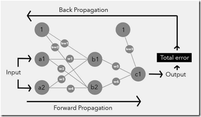
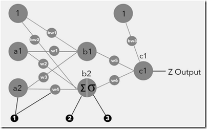
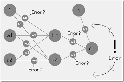
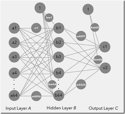
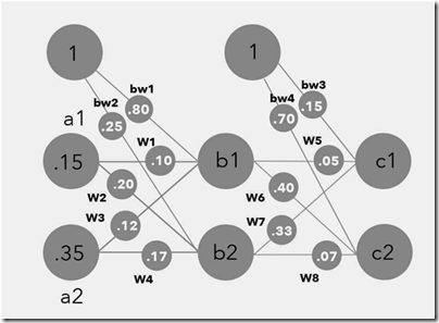
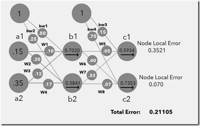
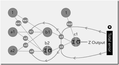
Well, in the context of ML, the application of Sigmoid curve is more practical. It can be used to replace the step function and suddenly things become more tractable. A single neuron can learn a straight line but a set of neurons, i.e multi-layer perceptron can learn more convoluted curves. Agreed there is a curse of dimensionality here, but if you think about it, the hyperspace explosion is a double edged sword. On the one hand, there objective function is far more wiggly but on the other hand, there is a less scope that you will stuck at a local minimum via gradient search methods. With this Sigmoid input and multi layer tweak, Perceptron came back with vengeance. There was a ton of excitement just like the time when perceptron was introduced. The algorithm by which the learning takes place is called "back propagation", a term that is analogous to how human brains work. This algo was invented by David Rumelhart in 1986. It is a variant of gradient descent method. There is no mathematical proof that Back propagation will find the global minimum/maximum, though. The backprop solves what the author calls "credit assignment" problem. In a multi-layered perceptron the error between the target value and the current value needs to be propagated across all layers backward. The basic idea of error propagation, i.e error assignment for each of the layers is done via backprop.

Whenever the learner’s "retina" sees a new image, that signal propagates forward through the network until it produces an output. Comparing this output with the desired one yields an error signal, which then propagates back through the layers until it reaches the retina. Based on this returning signal and on the inputs it had received during the forward pass, each neuron adjusts its weights. As the network sees more and more images of your grandmother and other people, the weights gradually converge to values that let it discriminate between the two.

Sadly the excitement phase petered down as learning with dozens of hundreds of hidden layers was computationally difficult. In the recent years though, backpropagation has made a comeback thanks to huge computing power and big data. It now goes by the technique "Deep Learning". The key idea of deep learning is based on auto encoders that is explained very well by the author. However there are many things that need to be worked out for deep learning to be anywhere close to the Master algorithm. All said and done there are a few limitations to exclusively following a connectionist tribe. Firstly, the learning algo is difficult to comprehend. It comprises convoluted connections between various neurons. The other limitation is that the approach is not compositional, meaning it is divorced from the way a big part of human cognition works.

 

Evolution : Nature’s Learning Algorithm

The chapter starts with the story of John Holland, the first person to have earned a PhD in computer science in 1959. Holland is known for his immense contribution to Genetic algorithms. His key insight lay in coming up with a fitness function that would assign a score to every program considered. What’s the role of fitness function ? Starting with a population of not-very-fit individuals-possibly completely random ones-the genetic algorithm has to come up with variations that can then be selected according to fitness. How does nature do that? This is where the genetic part of the algorithm comes in. In the same way that DNA encodes an organism as a sequence of base pairs, we can encode a program as a string of bits. Variations are produced by crossovers and mutations. The next breakthrough in the field of genetic programming came from Holland’s student John Koza who came up with the idea of evolving full blown computer programs.

Genetic programming’s first success, in 1995, was in designing electronic circuits. Starting with a pile of electronic components such as transistors, resistors, and capacitors, Koza’s system reinvented a previously patented design for a low-pass filter, a circuit that can be used for things like enhancing the bass on a dance-music track. Since then he’s made a sport of reinventing patented devices, turning them out by the dozen. The next milestone came in 2005, when the US Patent and Trademark Office awarded a patent to a genetically designed factory optimization system. If the Turing test had been to fool a patent examiner instead of a conversationalist, then January 25, 2005, would have been a date for the history books. Koza’s confidence stands out even in a field not known for its shrinking violets. He sees genetic programming as an invention machine, a silicon Edison for the twenty-first century.

A great mystery in genetic programming that is yet to be solved conclusively is the role of crossover. None of Holland’s theoretical results show that crossover actually helps; mutation suffices to exponentially increase the frequency of the fittest schemas in the population over time. There were other problems with genetic programming that finally made ML community at large divorce itself from this tribe

Evolutionaries and connectionists have something important in common: they both design learning algorithms inspired by nature. But then they part ways. Evolutionaries focus on learning structure; to them, fine-tuning an evolved structure by optimizing parameters is of secondary importance. In contrast, connectionists prefer to take a simple, hand-coded structure with lots of connections and let weight learning do all the work. This is machine learning’s version of the nature versus nurture controversy. As in the nature versus nurture debate, neither side has the whole answer; the key is figuring out how to combine the two. The Master Algorithm is neither genetic programming nor backprop, but it has to include the key elements of both: structure learning and weight learning. So, is this it ? Have we stumbled on to the right path for "Master Algorithm" ? Not quite. There are tons of problems with evolutionary algos. Symbolists and Bayesians do not believe in emulating nature. Rather, they want to figure out from first principles what learners should do. If we want to learn to diagnose cancer, for example, it’s not enough to say "this is how nature learns; let’s do the same." There’s too much at stake. Errors cost lives. Symbolists dominated the first few decades of cognitive psychology. In the 1980s and 1990s, connectionists held sway, but now Bayesians are on the rise.

 

In the Church of the Reverend Bayes

Perci Diaconis in his paper titled, MCMC Revolution, says that MCMC technique that came from Bayesian tribe has revolutionized applied mathematics. Indeed, thanks to high performance computing ability, Bayes is now a standard tool in any number cruncher’s tool kit. This chapter talks about various types of Bayesian techniques. The basic idea behind Bayes is that it is a systematic and quantified way of updating degrees of belief, in the light of new data. You can pretty much cast any problem, irrespective of the size of the data available, in to a Bayesian inference problem. Bayes theorem usually goes by the name "inverse probability" because in real life we know Pr(effect|cause) and we are looking to compute Pr(cause|effect). Bayes’ theorem as a foundation for statistics and machine learning is bedeviled not just by computational difficulty but also by extreme controversy. The main point of conflict between Bayesians and Non-Bayesians is the reliance of subjective priors to "turn on the Bayesian crank". Using subjective estimates as probabilities is considered sin by Frequentists, for whom, everything should be learned from the data.

One of the most common variant of Bayesian models is the "Naive Bayes" model where each cause is independent of other causes in creating an effect. Even though this assumption sounds extremely crazy, there are a ton of areas where Naive Bayes beats sophisticated models. No one is sure who invented the Naïve Bayes algorithm. It was mentioned without attribution in a 1973 pattern recognition textbook, but it only took off in the 1990s, when researchers noticed that, surprisingly, it was often more accurate than much more sophisticated learners. Also if you reflect a bit, you will realize that Naive Bayes is closely related to Perceptron algorithm.

The author mentions Markov Models as the next step in the evolution of Bayes models. Markov models are applicable to a family of random variables where each variable is conditionally independent of its history except the current state. Markov chains turn up everywhere and are one of the most intensively studied topics in mathematics, but they’re still a very limited kind of probabilistic model. A more complicated model is Hidden Markov Model where we don’t get to see the actual states but we have to infer them from the observations. A continuous version of HMM goes under the name "Kalman Filter" that has been used in many applications across domains.

Naive Bayes, Markov Models, Hidden Markov Models are all good but they are all a far cry from Symbolists. The next breakthrough came from Judea Pearl who invented Bayesian Networks. This allowed one to specify complex dependencies among random variables. By defining the conditional independence of a variable given a set of neighboring nodes, Bayesian networks tame the combinatorial explosion and make inferences tractable. Basically Bayesian Network can be thought of as a "generative model", a recipe for probabilistically generating a state of the world. Despite the complex nature of a Bayesian net, the author mentions that there have been techniques developed to successfully infer various aspects of the network. In this context, the author mentions MCMC and gives an intuitive explanation of the technique. A misconception amongst many is that MCMC is a simulation technique. Far from it, the procedure does not simulate any real process; rather it is an efficient way to generate samples from a Bayesian network. Inference in Bayesian networks is not limited to computing probabilities. It also includes finding the most probable explanation for the evidence. The author uses the "poster child" example of inferring the probability of heads from coin tosses to illustrate the Bayesian technique and compare it with the Frequentist world of inference.

The next set of models that came to dominate the Bayesian tribe is Markov Networks. A Markov network is a set of features and corresponding weights, which together define a probability distribution. Like Bayesian networks, Markov networks can be represented by graphs, but they have undirected arcs instead of arrows. Markov networks are a staple in many areas, such as computer vision. There are many who feel that Markov networks are far better than Naive Bayes, HMMs etc., as they can capture the influence from surroundings.

Bayesians and symbolists agree that prior assumptions are inevitable, but they differ in the kinds of prior knowledge they allow. For Bayesians, knowledge goes in the prior distribution over the structure and parameters of the model. In principle, the parameter prior could be anything we please, but ironically, Bayesians tend to choose uninformative priors (like assigning the same probability to all hypotheses) because they’re easier to compute with. For structure, Bayesian networks provide an intuitive way to incorporate knowledge: draw an arrow from A to B if you think that A directly causes B. But symbolists are much more flexible: you can provide as prior knowledge to your learner anything you can encode in logic, and practically anything can be encoded in logic-provided it’s black and white.

Clearly, we need both logic and probability. Curing cancer is a good example. A Bayesian network can model a single aspect of how cells function, like gene regulation or protein folding, but only logic can put all the pieces together into a coherent picture. On the other hand, logic can’t deal with incomplete or noisy information, which is pervasive in experimental biology, but Bayesian networks can handle it with aplomb.Combining connectionism and evolutionism was fairly easy: just evolve the network structure and learn the parameters by backpropagation. But unifying logic and probability is a much harder problem.

 

You are what you resemble

The author introduces techniques of the "Analogizers" tribe. This tribe uses similarities among various data points to categorize them in to distinct classes. In some sense, we all learn by analogy. Every example that illustrates an abstract concept is like an analogy. We learn by relating the similarity between two concepts and then figure what else one can infer based on the fact that two concepts are similar.

The chapter begins with explaining the most popular algorithm of the tribe, "the nearest neighbor algorithm". This was invented way back in 1951 by Evelyn Fix and Joe Hodges. The inventors faced a massive difficulty in publishing their algorithm. However the fact that the algo remained unpublished did not faze many researchers who went about developing variants of the algorithm like "K nearest neighbor" method, "Weighted K-nearest neighbor" etc. It was in 1967 that Tom Cover and Peter Hart proved that, given enough data, nearest-neighbor is at worst only twice as error-prone as the best imaginable classifier. This was a momentous revelation. Up until then, all known classifiers assumed that the frontier had a very specific form, typically a straight line. This was a double-edged sword: on the one hand, it made proofs of correctness possible, as in the case of the perceptron, but it also meant that the classifier was strictly limited in what it could learn. Nearest-neighbor was the first algorithm in history that could take advantage of unlimited amounts of data to learn arbitrarily complex concepts. No human being could hope to trace the frontiers it forms in hyperspace from millions of examples, but because of Cover and Hart’s proof, we know that they’re probably not far off the mark.

Is nearest neighbor algo, the master algorithm ? It isn’t because of curse of dimensionality. As the dimension of covariates goes up, the NN algo efficiency goes down. In fact the curse of dimensionality is the second most important stumbling block in the Machine learning, over-fitting being the first one. There are certain techniques to handle the dimension explosion but most of them are hacks and there is no guarantee that they are going to work.

Subsequently, the author introduces Support Vector Machines(SVM) that has become the most popular technique used by Analogizers. I loved the way author describes this technique using plain simple English. He asks the reader to visualize a fat serpent that moves between two countries that are at war. The story of finding the serpent incorporates pretty much all the math that is needed to compute support vectors, i.e.

• kernel for SVM
• support vectors
• weight of the support vectors
• constrained optimization
• maximizing the margin of the classifier

My guess is, one would understand the math far easier, after reading through this section on SVMs. SVMs have many advantages and the author highlights most of them. Books such as these also help us in verbalizing math stuff in simple words. For example, if you were to explain the difference between constrained optimization and unconstrained optimization to a taxi driver, how would you do it? Read this book to check whether your explanation is better than what the author provides.

Towards the end of the chapter, the author talks about case-based reasoning and says that in the years to come, analogical reasoning will become so powerful that it will sweep through all the fields where case-based reasoning is still employed.

 

Learning without a teacher

Unlike the previous chapters that focused on labeled data, this chapter is learning via unsupervised learning. Cognitive scientists describe theories of child learning using algos and machine learning researchers have developed techniques based on them. The author explains k-means algorithm, a popular clustering technique. It is actually a special case of Expectation Maximization(EM) algorithm that was invented by three Harvard statisticians. EM is used in a ton of places. To learn hidden Markov models, we alternate between inferring the hidden states and estimating the transition and observation probabilities based on them. Whenever we want to learn a statistical model but are missing some crucial information (e.g., the classes of the examples), we can use EM. Once you have a cluster at the macro level, nothing stops you from using the same algo for each cluster and come up with sub-clusters etc.

Subsequently, the author introduces another popular technique for unsupervised learning, PCA, that is used for dimensional reduction. PCA tries to come up linear combination of various dimensions in the hyperspace so that total variance of the data across all dimensions is maximized. A step up to this algo is called "Isomap", a nonlinear dimensionality reduction technique. It connects each data point in a high-dimensional space (a face, say) to all nearby points (very similar faces), computes the shortest distances between all pairs of points along the resulting network and finds the reduced coordinates that best approximate these distances.

After introducing clustering and dimensional reduction techniques, the author talks about "Reinforcement learning", a technique that relies on immediate response of the environment for various actions of the learner. Research on reinforcement learning started in earnest in the early 1980s, with the work of Rich Sutton and Andy Barto at the University of Massachusetts. They felt that learning depends crucially on interacting with the environment, but supervised algorithms didn’t capture this, and they found inspiration instead in the psychology of animal learning. Sutton went on to become the leading proponent of reinforcement learning. Another key step happened in 1989, when Chris Watkins at Cambridge, initially motivated by his experimental observations of children’s learning, arrived at the modern formulation of reinforcement learning as optimal control in an unknown environment. A recent example of a successful startup that combines neural networks and reinforcement learning is "DeepMind", a company that was acquired by Google for half a billion dollars.

Another algorithm that has a potential to be a part of "Master Algorithm" is chunking. Chunking remains a preeminent example of a learning algorithm inspired by psychology. The author gives a basic outline of this concept. Chunking and reinforcement learning are not as widely used in business as supervised learning, clustering, or dimensionality reduction, but a simpler type of learning by interacting with the environment is: A/B testing. The chapter ends with the author explaining another potentially killer algo, "relational learning".

 

The Pieces of the Puzzle Fall into Place

Progress in science comes from unifying theories; two or more seemingly disparate observations are driven by the same logic or law. If one looks at ML, it appears that Master Algorithm is akin to a unifying theory in science. It will unify all the master algorithms of each tribes, all the techniques of each tribes and give one cohesive way to learn from data.

In fact there is already a technique called "meta learning" that some of the tribes use with in their techniques. For example, bagging, random forests and boosting are some of the famous meta learning techniques used by Symbolists. Bayesians have something called "model averaging" that learns from each model by considering it as an hypothesis and then computes a score based on the vote given by each of the models. Meta learning in its current avatar is remarkably successful, but it’s not a very deep way to combine models. It’s also expensive, requiring as it does many runs of learning, and the combined models can be quite opaque.

The author used the following schematic diagram for each of the tribes, while explaining the rationale of a possible “Master Algorithm”

He then takes the reader through a tour of each of the tribes philosophy and their master algorithms and comes up a unifier, called "Alchemy", that he calls it as the "Master Algorithm". In the process of creating this master algorithm, he introduces Markov Logic Networks and says that they serve for representing the problem. Alchemy uses posterior probability as the evaluation function, and genetic search coupled with gradient descent as the optimizer. The author is wary about Alchemy’s immediate application and says that there is a ton of research that is yet to be done, so that it can become a true Master Algorithm, i.e., one that has the capability to solve hard problems.

This chapter is a little more involved as it tries to connect all the ideas from the previous eight chapters and introduces a way to combine the various pieces of puzzle to create a "Master Algorithm". The chapter will also be very interesting for an aspiring ML researcher  who is trying to pick his focus area.

 

This is the World on Machine Learning

The last chapter of the book discusses the world in which "Master Algorithm" is all pervasive. The author tries to speculate answers to the following questions :

• Will humans be replaced by machines ?
• What do you want the learners of the world to know about you ?
• How good a model of you, a learner, can have ?
• How will ecommerce shopping experience be ?
• Will there be a rise of "humanities" disciple after the automation of most of non-human related tasks ?
• What will the current online dating sites morph in to ?
• How will the Amazons, Netflixes, Googles of the world change ?
• What will be the privacy issues in a society where most of the transactions and activities involve, one algo talking to another algo?
• Will future wars be fought by robots ?
• Will robot-warfare be viable ?
• Will AI and Master Algorithm take over the world ?

The author ends the book by saying,

Natural learning itself has gone through three phases: evolution, the brain, and culture. Each is  product of the previous one, and each learns faster. Machine learning is the logical next stage of this progression. Computer programs are the fastest replicators on Earth: copying them takes  only a fraction of a second. But creating them is slow, if it has to be done by humans. Machine learning removes that bottleneck, leaving a final one: the speed at which humans can absorb change.

Takeaway :

This book is a pop-science book for Machine Learning. ML has reached a point where it is not just for geeks anymore. Every one needs to know about it, Every one needs to at least have a conceptual model about the field as it has become all pervasive. Having said that, it would take time to plod though the book if you are a complete newbie to ML. This book is massively appealing to someone who a cursory knowledge of a few ML techniques and wants to have a 10,000 ft. view of the entire fields’ past, present and future. The future, as the title of book states is, would be the invention of a master algorithm that unifies methods across all the five tribes.

 

Bayes’ Rule – A Tutorial Introduction to Bayesian Analysis : Book Review

The book serves a nice intro to Bayes theory for an absolute newbie. There is minimal math in the book. Whatever little math that’s mentioned, is accompanied by figures and text so that a newbie to this subject “gets” the basic philosophy of Bayesian inference. The book is a short one spanning 150 odd pages that can be read in a couple of hours.  The introductory chapter of the book comprises few examples that repeat the key idea of Bayes. The author says that he has deliberately chosen this approach so that a reader does not miss the core idea of the Bayesian inference which is,

Bayesian inference is not guaranteed to provide the correct answer. Instead, it provides the probability that each of a number of alternative answers is true, and these can then be used to find the answer that is most probably true. In other words, it provides an informed guess.

In all the examples cited in the first chapter, there are two competing models. The likelihood of observing the data given each model is almost identical. So, how does one chose one of the two models ? Well, even without applying Bayes, it is abundantly obvious which of the two competing models one should go with. Bayes helps in formalizing the intuition and thus creates a framework that can be applied to situations where human intuition is misleading or vague. If you are coming from a frequentist world where “likelihood based inference” is the mantra, then Bayes appears to be merely a tweak where weighted likelihoods instead of plain vanilla likelihoods are used for inference.

The second chapter of the book gives a geometric intuition to a discrete joint distribution table. Ideally a discrete joint distribution table between observed data and different models is the perfect place to begin understanding the importance of Bayes. So, in that sense, the author provides the reader with some pictorial introduction before going ahead with numbers. 

The third chapter starts off with a joint distribution table of 200 patients tabulated according to # of symptoms and type of disease. This table is then used to introduce likelihood function, marginal probability distribution, prior probability distribution, posterior probability distribution, maximum apriori estimate . All these terms are explained using plain English and thus serves as a perfect intro to a beginner. The other aspect that this chapter makes it clear is that it is easy to obtain probability of data given a model. The inverse problem, i.e probability of model given data, is a difficult one and it is doing inference in that aspect that makes Bayesian inference powerful. 

The fourth chapter moves on to  continuous distributions. The didactic method is similar to the previous chapter. A simple coin toss example is used to introduce concepts such as continuous likelihood function,  Maximum likelihood estimate, sequential inference, uniform priors, reference priors,  bootstrapping and various loss functions.

The fifth chapter illustrates inference in a Gaussian setting and establishes connection with the well known regression framework. The sixth chapter talks about joint distributions  in a continuous setting.  Somehow I felt this chapter could have been removed from the book but I guess keeping with the author’s belief that “spaced repetition is good”, the content can be justified. The last chapter talks about Frequentist vs. Bayesian wars, i.e. there are statisticians who believe in only one of them being THE right approach. Which side one takes depends on how one views “probability” as – Is probability a property of the physical world or is it a measure of how much information an observer has about that world ? Bayesians and increasingly many practitioners in a wide variety of fields have found the latter belief to be a useful guide in doing statistical inference. More so, with the availability of software and computing power to do Bayesian inference, statisticians are latching on to Bayes like never before.

The author deserves a praise for bringing out some of the main principles of Bayesian inference using just visuals and plain English. Certainly a nice intro book that can be read by any newbie to Bayes.

 

Queueing Systems : Volume I

 

A document containing brief summary of the book

 

Takeaway :

This book is a beautiful book that describes the math behind queueing systems. One learns a ton of math tools from this book, that can be used to analyze any system that has a queueing structure within it. The author presents the material in a highly enthusiastic tone with superb clarity. Thoroughly enjoyed going through the book.

 

Quantitative Trading with R : Book Review

A brief summary of the book

 Takeaway :

The book is definitely overpriced for what it delivers. Given that 50% of this book explains R basics, the title is not at all appropriate. Even the quant stuff that is covered in the remaining 50% of the book is laughably inadequate.

 

Digital Dice : Book Review

In the last few decades, enormous computational speed has become accessible to many. Modern day desktop has good enough memory and processing speed that enables a data analyst to compute probabilities and perform statistical inference by writing computer programs. In such a context, this book can serve as a starting point to anyone who wishes to explore the subject of computational probability. This book has 21 puzzles that can be solved via simulation.

Solving a puzzle has its own advantages. Give a dataset with one dependent variable and a set of predictors to a dozen people asking them to fit a regression model; I bet that you will see at least a dozen models, each of which could be argued as a plausible model. Puzzles are different. There are constraints put around the problem that you are forced to get that ONE RIGHT solution to the problem. In doing so, you develop much more sophisticated thinking skills.

In the introductory chapter of the book, the author provides a basic framework for computational probability by showing ways to simulate and compute probabilities. This chapter gives the reader all the ammunition required to solve the various puzzles of the book. The author provides detailed solutions that includes relevant MATLAB code, to all the 21 puzzles.

Some of my favorite puzzles from the book that are enlightening as well as paradoxical are :

• ˆ The Gamow-Stern Elevator
• ˆ The Pipe Smoker’s Discovery
• ˆ A Toilet Paper Dilemma
• ˆ Parrondo’s Paradox
• ˆ How Long Is the Wait to Get the Potato Salad ?
• ˆ The Appeals court Paradox

Here is the link to my document that flushes out the details of all the 21 puzzles in the book:

Digital Dice – Solving Puzzles with R

What’s in the above document?

I have written R code that aims to computationally solve each of the puzzles in the book. For each puzzle, there are two subsections. First subsection spells out my attempt at solving the puzzle. The second subsection contains my learning from reading through the solution given by the author. The author provides extremely detailed MATLAB code that anyone who has absolutely no exposure to MATLAB can also understand the logic. In many cases I found that the code snippets in the book looked like elaborate pseudo code. There are many good references mentioned for each of the puzzles so that interested readers can explore further aspects. In most of the cases, the reader will realize that closed form solutions are extremely tedious to derive and simulation based procedures make it easy to obtain solutions to many intractable problems.

 

Difference and Differential Equations with Applications in Queueing theory : Book Review

In a book that has about 350 pages, the first 250 odd pages are devoted to probability, ODEs and difference equations. The last part of the book covers queuing theory for specific systems, i.e, Poisson arrivals, exponential service times of one or more servers. The most painful thing about this book is that there are innumerable typos. A book that is riddled with typos on almost every other page cannot be an appealing text for an undergrad.  My guess is that, this book will be never make it to an undergrad’s study table, unless the authors make a serious effort to publish an errata or come up with a better version of the book. Is there anything good about the book at all ? Well, may be, the chapter on difference equations is worth going over just once. On a second thought, I think that the first 250 pages of the book can be rewritten concisely so that it can be pushed to the appendix.  That leaves the last 100 pages of the book that reads more like a cheat sheet rather than a book from which one can really learn something. This book desperately needs a rewrite from the authors,else it is going to languish alongside the books that die silently every year.