Doing Bayesian Data Analysis : Summary

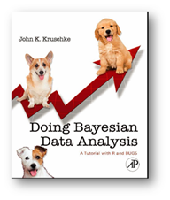
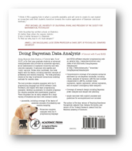
Firstly, something about the puppies on the cover pages. The happy puppies are named Prior, Likelihood, and Posterior. Notice that the Posterior puppy has half-up ears, a compromise between the perky ears of the Prior puppy and the floppy ears of the Likelihood puppy. The puppy on the back cover is named Evidence. MCMC methods make it unnecessary to explicitly compute the evidence, so that puppy gets sleepy with nothing much to do. These puppy images basically summarize the essence of Bayes’ and MCMC methods.

I was tempted to go over the book after reading the preface of the book where the author writes candidly about, “What to expect from the book?”.He uses poetic verses, humor to introduce the topic. He promises the usage of simple examples to explain the techniques of Bayesian analysis. The book is organized in to three parts. The first part contains basic ideas on probability, models, Bayesian reasoning and R programming. So, I guess this part could be speed read. The second part is the juicy part of the book where simple dichotomous data is used to explain hierarchical models, MCMC, sampling methods, Gibbs sampler and BUGS. The third part of the book covers various applications of Bayesian methods to real life data. So, this is more like a potpourri of applications and a reader can pick and choose whichever application appears exciting / relevant to one’s work. The highlight of this book is it enables you to DO Bayesian analysis, and not just KNOW about Bayes’. The book also gives an analogue for each of the tests that one learns in NHST( Null Hypothesis Significance testing). Historically Bayesians have always scorned at tests based on p-values. The inclusion of the tests in the book shows the author’s willingness to discuss issues threadbare and highlight the flaws in using frequentist tests for real life data.

Something not related to this post – I wonder how many Statistics courses in Indian universities teach Bayes to students. Historically Bayes became popular in Bschools . It was only after it was absorbed by BSchools, that it was then was adopted in other disciplines. Considering this sequence of events, I really doubt whether Bschools in India ever think of highlighting atleast a few case studies based on Bayes. As far as my experience goes, Bschools scare the students with boring statistical techniques which are outdated. Andrew Gelman wrote a fantastic book titled, “A bag of tricks? ”. I will blog about it someday. The book has fantastic content that can be used to structure any statistics based course at BSc/MBA level. But how many faculty even bother to do such things ? What matters is that a few faculty personnel who have the courage to change the curriculum and teach what is relevant in statistics, than merely following the traditional frequentist ideas. If you take a random sample of students from any Bschool in India  and ask them whether they remember anything from statistics courses, I bet they would say, “Yeah it was something about pvalues , null hypothesis and something hypothesis testing”. Sadly, this reflects the state of our education system as it has failed miserably to inculcate statistical thinking amongst students. Anyways enough of my gripe, Let me get back to the intent of the post.

As I mentioned earlier, the Part I of the book can be quickly read and worked on. There is one thing worth mentioning about the first part of the book. The way in which Bayes’ is introduced is very intuitive and by far the easiest to visualize, out of all the intros I have read till date. Well, one comes across Bayes’ in some form or the other be it through Monty-Hall problem/ conditional probability problems etc. This is the first time I am coming across where Bayes’ is introduced from a Contingency table perspective. If you look at a contingency table and assume that rows represent various data realizations and columns represent parameter realizations, then one can formulate the Bayes’ theorem quite easily. Conditioning on the data is equivalent to restricting the attention to one row and Bayes probabilities are nothing but reevaluated probabilities in that row, based on the relative proportions of the probabilities appearing in the row. One new term that I got to learn from this chapter is “evidence” and the way it is used in relation to Bayes. The denominator appearing in Bayes is termed as evidence. The “evidence”, is the probability of the data according to the model, determined by summing across all possible parameter values weighted by the strength of belief in those parameter values. In other books, “evidence” is the called “prior predictive”. Another important aspect mentioned is Data order invariance, meaning the likelihood is independent and identically distributed.The likelihood function has no dependence on time ordering and thus is time invariant.

Part II of the book is the core of the book where all the fundamentals are applied to Inferring a Binomial Proportion. Most of algorithms are applied to a simple case of dichotomous data so that the reader gets an intuitive understanding as well as working knowledge of these algorithms.

Inferring Binomial Proportion Via Exact Mathematical Analysis

By taking beta as a prior distribution for binomial likelihood, one gets the posterior as beta distribution. Based on one’s belief one can choose the values of a & b to reflect the bias in the coin. Highly skewed priors can be represented with values of a and b less than 1, for uniform priors, one can take a=b=1, for skewed on one side priors, one can take the prior as a=100,b=1 or a=1, b=100 and for a fair coin, one can take a=b=some high value. So, specifying beta prior is a way to translate the beliefs in to quantitative measure.

The three goals of inference are 1) estimating the parameter of binomial proportion, 2) predicting the data , 3) model comparison. For the first goal, a credible interval is computed based on the posterior distribution. Predicting the data can be done using the expectation rule on posterior distribution. The third goal is tricky. Only a few guidelines are given, one being the computation of Bayes’ factor.

If there are two competing models, meaning two competing priors for the data, then one can use Bayesian inference to evaluate the two models. One needs to calculate the probability of evidence for both the models i.e calculate Bayes factor P(D/M1) / P(D/M2). If this factor is extremely small / big, one can get an idea that Model 1/ Model 2 is better. Let’s say the ratio is very close to 0. Based on this evaluation, one cannot come to conclusion that Model M1 is better. The model comparison process has merely told us the models’ relative believabilities, not their absolute believabilities. The winning model might merely be a less bad model than the horrible losing model.

Steps to check winning model robustness (Posterior predictive check )

1. Simulate one value for the parameter from the posterior distribution
2. Use that parameter to simulate data values
3. Calculate the proportion of wins
4. Repeat these steps million times and check whether the probability of evidence is big enough

It is possible that Best model of the competing models might be a less bad model than the horrible losing model. Basically this chapter gives the first flavor of using Bayes’ with using a known closed form conjugate prior for computing the posterior probability model.

Inferring Binomial Proportion through Grid approximation:

The chapter then talks about a method that frees the modeler from choosing only closed form priors. The prior need not be a closed form distribution such as beta but might as well be tri-modal/ discrete mass function. In all probability, the real life prior would mostly be a discrete mass function for binomial proportion estimation. Prior distributions for binomial parameter estimation thus will have some discrete values with some specific probability values. One can think of triangular, quadratic, parabolic, whatever discrete prior that you can think of. The beauty of the grid method is that you can evaluate the probability at each of the grid value and then multiply that probability by the likelihood function for that point on the grid. This gives the posterior probability for the same point on the grid. The grid method has another advantage, i.e the calculation of HDI( Highest density Interval) that is a discrete approximation. Estimation + Prediction + Model Evaluation are applied to dichotomous data to show the application of grid based method. The grid method thus is an amazing way to incorporate subjective beliefs in to the prior and compute the HDI for the binomial proportion.

Inferring Binomial Proportion Via Metropolis Algorithm:

Nicholas Metropolis published the algorithm in 1953

The methods introduced in the previous chapters involve specifying the prior that are in closed form, or priors that can be specified in a discrete form on a grid. However if the parameters explode, the number of grid points that one needs to evaluate grows exponentially. If we set up a grid on each parameter that has 1,000 values, then the six dimensional parameter space has 1,000^6 = 1,000,000,000,000,000,000 combinations of parameter values, which is too many for any computer to evaluate.

One can use Metropolis Algorithm or invoke the necessary functions in BUGS to sample values from the posterior distribution. The condition that, “ P(theta) and P(evidence/theta) can be computed at every theta “ is enough to generate sample values from the posterior distribution. The metropolis algorithm is introduced via “Politician visit example”, a simple but powerful example of showing the internals of Metropolis algorithm. Even though Metropolis is almost never used to infer binomial proportion, the example builds a solid intuition in to working of Metropolis.

The main components of Metropolis algorithm applied to the simple example are

• Proposal distribution
• Target distribution ( Typically the product of likelihood and prior )
• Burn rate ( what % of the initial random walk should be abandoned ?)

One can also form a transition matrix which gives an intuition on,” Why the random walks converge to the target distribution? “, “ Why does the repeated multiplication of transition matrix converge to a stable matrix? ”. One thing to keep in mind about Metropolis algorithm is that prior and likelihood need not be normalized probability distributions, all that matters is the ratio of target probabilities of proposed and current probabilities. The book says it better, “The Metropolis algorithm only needs the relative posterior probabilities in the target distribution, not the absolute posterior probabilities, so we could use an unnormalized prior and/or unnormalized posterior when generating sample values of θ”

One must however keep in mind that, Proposal distributions can take many different forms, but the goal should be to use a proposal distribution that efficiently explores the regions of the parameter space where probability has most of its mass. MCMC methods have revolutionized Bayes’ methods and Metropolis algorithm is an example of one. Computation of evidence is the toughest part of Bayesian analysis. Hence MCMC methods can be used to solve this specific kind of problem. Thus “politician example”, mentioned in the book is a good introduction to Markov Chain Monte Carlo methods.

Basic Intro to BRugs

For the metropolis to work, the following conditions become crucial

• The proposal distribution needs to be tuned to prior distribution
• Initial samples during the burn-in-period needs to be excluded
• Sampling chain needs to be run long enough

These issues are taken care of by using BUGS package. Now to use BUGS, one needs a wrapper so that R can communicate with BUGS. There are different BUGS versions for windows, linux and other open source softwares. OpenBUGS is used in this book for specifying Bayesian models and generating MCMC. The wrapper that is used to communicate R with OpenBUGS is BRugs package. I am using a 64 bit machine and it was particularly painful to know that BRugs is available only for 32 bit machines. So, the code I wrote had to be configured to talk to 32 bit installation of R so that BRugs could be invoked. BTW, it requires a 32 bit JRE if you are working with eclipse.

The syntax for OpenBUGS is somewhat similar to R , so learning curve is not so much. Infact all one needs to know atleast for preliminary applications is the way to specify, likelihood, prior and the data realization. The chapter does a fantastic job of showing the way to use OpenBUGS from R. modelData(), modelCompile(),modelGenInits(),modelUpdate() are the main functions in BRugs to put data in to model, to compile the model, to initialize the chain and creating a MCMC chain. All these function details are already coded in BUGS can be leveraged using BRugs wrapper.BUGS can also be used for prediction and model comparison.

The highlight of this chapter is the application of Metropolis to single parameter estimation. Typically Metropolis is used only for multi parameter estimation and hence is usually introduced in any book after significant material is covered. By applying Metropolis to a simple example where the proposal distribution takes only 2 values, a lot of things get intuitively clear for the reader.

Also the extensive R code provided for Metropolis algorithm, computing HDI, invoking BUGS using BRugs is extremely useful to get a feel of the workings. The code is extremely well documented and the fact that they are part of the chapter itself makes the chapter a self-contained one.

Inferring Binomial Proportion Via Gibbs Sampling Algorithm:

Stuart Geman and Donald Geman were enthused on Bayes’ application to Pattern recognition after attending a seminar. They both went on to invent a technique called “Gibbs Sampling Method”

Stuart Geman Donald Geman

In any real life modeling problem one needs to deal with multiple parameters and one needs a methods for doing Bayesian analysis. BUGS( Bayes using Gibbs sampler) provides powerful software to carry out these analysis.

What is Gibbs Sampling ? You consider the parameters to be estimated , let’s say theta_1, theta_2,…theta_n. Select a theta_i from the list and generate a random value for the parameter from the conditional distribution of theta_i given other thetas. This procedure is repeated in a cyclical manner for all the thetas until you get to the target distribution. In Metropolis, the proposed jump affects only one parameter at a time, and the proposed jump is sometimes rejected, unlike Gibbs sampling where the proposed jump is never rejected. Gibbs Sampling is extremely efficient algorithm when it can be done, but the sad part is that it cannot be done in all the cases.

The thing about multiple parameter is that to look at the probability distribution you need a 3d plot, or a projection on a 2d surface. So, the chapter starts off with giving some fundas about basic plots using contour and persp functions in R package. One needs to know “outer” function in R to plot these 3d plots. The chapter starts off with deriving posterior for a two parameter case using formal analysis. The prior, likelihood and posterior are displayed using persp and countour plot. Grid method is used when the prior cannot be summarized by a nifty function. Let’s say you have prior function that looks like ripples and you want to estimate the posterior. One can easily form a grid, evaluate the prior at each point, evaluate the likelihood at each point and multiply both to get the posterior distribution.

So, if grid methods or closed form prior methods do not work ( in the case of multiple parameter) , one can use Metropolis algo where you choose a prior, select a burnout period, select a likelihood function and use BUGS/ R code to generate the posterior distribution. So, if there are already three methods , what the advantage of Gibbs sampling ? Answer : One can ignore the effort that goes in to tuning the prior distribution.

The procedure for Gibbs sampling is a type of random walk through parameter space,like the Metropolis algorithm. The walk starts at some arbitrary point, and at each point in the walk, the next step depends only on the current position, and on no previous positions.Therefore, Gibbs sampling is another example of a Markov chain Monte Carlo process.What is different about Gibbs sampling, relative to the Metropolis algorithm, is how each step is taken. At each point in the walk, one of the component parameters is selected. The component parameter can be selected at random, but typically the parameters are cycled through, in order: θ1, θ2, θ3, . . . , θ1, θ2, θ3, . . .. (The reason that parameters are cycled rather than selected randomly is that for complex models with many dozens or hundreds of parameters, it would take too many steps to visit every parameter by random chance alone, even though they would be visited about equally often in the long run.) Gibbs sampling can be thought of as just a special case of the Metropolis algorithm, in which the proposal distribution depends on the location in parameter space and the component parameter selected. At any point, a component parameter is selected, and then the proposal distribution for that parameter’s next value is the conditional posterior probability of that parameter. Because the proposal distribution exactly mirrors the posterior probability for that parameter, the proposed move is always accepted.

The place where Gibbs sampling is extremely useful is when it is difficult to estimate the joint distribution but it is easy to estimate the marginal distribution of each parameter. Advantage big advantage of Gibbs sampling is that there are no rejected simulations unlike the Metropolis algorithm. Thus the basic advantage of Gibbs sampling over the Metropolis algorithm, is that there is no need to tune a proposal distribution and no inefficiency of rejected proposals. But there is one other disadvantage of Gibbs sampling. Because it only changes one parameter value at a time, its progress can be stalled by highly correlated parameters.

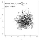
A visual to illustrate what’s wrong with Metropolis incase one doesn’t tune the proposed distribution properly. Incase you choose the proposed distribution with low standard deviation, the path just gets stagnated at a local point (fig. on left) . If you choose the proposed distribution with high probability, the most of the jumps are ignored(fig. in the center). The key is to use the correct the proposed distribution so that the chain generated is long enough and wanders enough to get suitable values from the posterior distribution(fig.on the right)

The above visual makes a strong case to trust MCMC in BUGS instead of Metropolis algorithm where the modeler might not be sure about the proposal distribution.

Bernoulli Likelihood with Hierarchical Prior

Dennis V Lindley Adrian F. Smith

Lindley and his student Adrian F Smith were the first scientists who showed Bayesians the way to develop hierarchical models. The hierarchical models fell flat in the face as the models were too specialized and stylized for many scientific applications. It would be another 20 years before students began their preliminary understanding of Bayes’ by looking in to hierarchical models. The main reason Hierarchical models became workable was “the availability of computing power”.

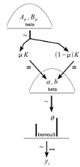
This chapter is all about Hierarchical models and applying various techniques for parameter inference. The chapter starts off with an example where the binomial proportion parameter of a coin depends on another parameter(hyperparameter). This hyperparameter is a beta distribution and the dependency between hyperparameter and parameter is through a constant K. Looking at the figure on the left mu is the hyperparameter, theta is the parameter and K is the constant that decides the dependency between mu and theta. For large values of K, there is a strong dependency as the resulting beta distribution is very narrow , whereas for small values of K, there is a weak dependency as the resulting beta is flat. One thing to notice is that there is no need for any hierarchical modeling if K takes a very high value or mu takes only one value. In both these situations the uncertainty of theta is captured in only one level. The first approach explored is the grid approach. Basically you divide the parameter space in to fine grids, formulate priors and joint priors, multiply by joint likelihood and you obtain a join posterior.

This is further extended to a series of coins and this where one sees that plain vanilla grid approach fails spectacularly. For a 2 coin experiment, it is still manageable but once we go on to 3 coin model, the grid points explodes to 6.5 million(on a 50 point grid for each param). It explores to 300 million for a 4 coin model. Hence this approach even though appealing and simple in one way becomes inefficient as the parameter space widens even a bit. MCMC comes to the rescue again. BUGS is then used to estimate parameters for more than 2 coins. The approach followed is , write BUGS code , wrap in a string, use BRugs package to interact with BUGS, simulate the MCMC chain , get the results from BUGS and analyze the result. BUGS gives an enormous flexibility. One can even include K as a parameter instead of fixing it. The chapter then introduces modeling a bigger parameter space.. It ends with a case study where Hierarchical models are applied to a real life situation.

The problem with examples mentioned are BRUGS is that it works with OpenBUGS that is available for a 32 bit machine. My machine is 64 bit and I had to do some acrobatics to make the examples work. I used RStudio which has a 32 bit R version and 32 bit JRE and then tried running the whole stuff. Even though I could run the code, I could never understand stuff as I was struggling to code. That’s when I stumbled on R2WinBUGS which had a wrapper to WinBUGS. I am relieved that I can now run R code to interact with WinBUGS with out having to worry about 32bit/62 bit constraint. Once I figured out the way to code almost everything in R and use R2WInBUGS to run MCMC sampling, working on Hierarchical models was a charm. While experimenting various software and packages, here are a few things I learnt :

• BRUGS works with OpenBUGS. All the functions in BRUGS replicate the interface functions in WINBUGS software. BRUGS works for 32 bit machine and not 64 bit machine
• OpenBUGS is published under GPL. It runs on Linux too. Provides a flexible API so that BRUGS can talk to OpenBUGS
• "“coda” package is used to analyze WinBUGS output.
• JAGS – Just another Gibbs Sampler : Alternative to the existing versions in WinBUGS/ OpenBUGS. It is used to run with coda and R
• R2WinBUGS – Interface written by Gelman to interact with WinBUGS. The main functions of R2WinBUGS are bugs() , bugs.data.inits(), bugs.script(), bugs.run(), bugs.sims()
• It’s better to code the model in WinBUGS , check the basic syntax of the model and then code the whole thing in R

Thinning is another aspect that is discussed in the chapter. Since posterior distribution samples are dependent, it is important to reduce the autocorrelation amongst the samples. This is used by specifying the thinning criteria where the samples are selected after some lag.

Hierarchical Modeling and Model Comparison

This chapter talks about model comparison, meaning if you specify two or more competing priors, on what basis does one choose the model ?

For comparing two models, an elementary approach is used to give an intro. Let’s say one is not certain about the binomial proportion parameter and chooses to have a discrete prior with two peaks at 0.25 and 0.75. One can use the code the model in WinBUGS in such a way that posterior samples are generated from these two priors at once. So, one simulation gives out the conditional probability values of both the models. These posterior probability values can be then used to judge the competing models. The chapter then goes on to use pseudo priors and shows a real life example where Bayes’ can be used to evaluate competing models/priors.

 

Null Hypothesis Significance Testing

Ronald Aylmer Fisher

It was Fisher who introduced p values, which became the basis for hypothesis testing for many years. Now how do we tackle this issue in this new world where there is no paucity of data, amazing visualization tools and computational power. What has Bayes’ got to offer in this area ?

The chapter is extremely interesting for any reader who wants to compare the frequentist methods to Bayesian approaches. The chapter starts with ripping apart the basic problem with NHST. From a sample of 8 heads out of 23 flips, the author uses NHST to check whether the coin is biased. In one case, he says the experimenter had a fixed N in mind which leads to rejection of alternate hypothesis, while in the second case the experimenter was tossing the coin until 8 heads appeared, in which case NHST leads to rejecting the null hypothesis. Using this simple example the author makes a point that the inference is based on the intention of the experimenter which the realized data will never be able to tell. This dependence of the analysis on the experimenter’s intentions conflicts with the opposite assumption that the experimenter’s intentions have no effect on the observed data. So, NHST in that way looks dicey for application purposes. Instead of tossing coins, if we toss flat headed nails and assume that tails means nail falls on the ground and heads is the alternate case, then NHST gives the same result even though our prior about flat headed nails is that the parameter is strongly biased towards tails. NHST gives no way of incorporating prior beliefs in to the modeling process. So, in a lot of cases it really becomes a tool which gives nonsense results.

The same kind of reasoning holds good for confidence intervals. Based on the covert intention of the experimenter, the confidence intervals could be entirely different for the same data. On the other hand, Bayesian Highest Density Interval is very clear to understand. It has direct interpretation of the believabilities of theta. It has no dependence on the intention of the experimenter and it is responsive to analyst’s prior beliefs. The chapter ends with giving a few advantages of thinking about sampling distribution.

Bayesian Approached to Testing a Point(“Null”) Hypothesis:

The way to test the null hypothesis is to check whether the null point falls within the credible interval. One important point mentioned in this context is that one must not be blinded by visual similarity between marginal distributions of two parameters and infer that they are same. It might so happen that they might be positively correlated in the joint behavior and the credible interval for the difference in the parameters might not contain 0. Instead of inferring that the two parameters are different, visual similarity might blind us to infer that they are the same. I came across another term in the chapter for the first time till date, Region of Practical Equivalence(ROPE). Instead of checking whether null value lies in the credible interval, it is better to check whether the an interval around null value , i.e whether ROPE comprises the credible interval or not?. By talking about ROPE instead of a single point, we are basically cutting down the false alarm rate. To summarize, a parameter value is declared to be accepted for practical purposes, if that value’s ROPE completely contains the 95% HDI of the posterior of the parameter.

Part III of the book that talks about model building, more specifically GLM

The Generalized Linear Model

The entire structure of modeling that is usually found in statistics 101 courses is based on Generalized Linear Model structure. In such a structure, you typically find predictor and predicted variable linked by a function. Depending on the type of predictors and the functions, GLM model goes by a different name. If the predictors and predicted variable are metric scale variable, then GLM usually goes by the name, “Regression” / “Multiple Regression”. If the predictor is nominal then it is recoded as appropriate factors and then fed in to the usual regression equation. There are cases when predicted variable is connected to the predictors using a link function. Typically this takes the form of sigmoid(logit), cumulative normal etc. Sigmoid is used when the predicted variable takes values between 0 and 1. The various illustrations to show the effect of gain + threshold + steepness in a sigmoid function are very helpful to any reader to get an idea of various GLM models possible.

The following is the usual form of GLM

The mean of the predicted variable is a function (f) of predictors(x1, x2,..) where f is termed as the link function. The predicted variable is in turn modeled as a pdf with the above mean and a precision parameter. Various forms of GLM models are an offshoot of the above structure. Typically f is Bernoulli / sigmoid/ constant / cumulative normal function. Various chapters in the part III of the book are organized based on the form f takes and the type of predictors + predicted.Chapter 15 is Bayes’ analogue of t-test. Chapter 16 is the Bayes’ analogue of Simple linear regression. Chapter 17 is the Bayes analogue of Multiple Regression. Chapter 18 is the Bayes analogue of One-way Anova. Chapter 19 is the Bayes’ analogue of two way ANOVA. Chapter 20 deals with logistic regression.

I will summarize the last part of the book (~200 odd pages) in another post at a later date. The first two parts of the book basically provide a thorough working knowledge of the various concepts in Bayesian Modeling. In fact a pause after marathon chapters of part I and part II of the book might be a better idea as one might need some time to reflect and link the concepts to whatever stats ideas that one already has.

Takeaway

The strength of this book is its simplicity. The book is driven by ONE estimation problem, i.e, inferring a binomial proportion. Using this as a “spine”, the author shows a vast array of concepts / techniques / algorithms relevant to Bayes’. In doing so, the author equips the reader with a working knowledge of Bayesian models. The following quatrain from Prof. McClelland (Stanford) on the cover of the book tells it all :

John Kruschke has written a book on Statistics
Its better than others for reasons stylistic
It also is better because it is Bayesian
To find out why, buy it – its truly amazin!